Placing your bets in weather forecasting

Expand all detail boxes for printing

Which approaches can create high-performing models? - While there is no clear answer to this, it is clear that exhaustive optimization of every modeling facet is unlikely to be the right choice. Often, it is enough to apply a handful of methodological tricks in combination with carefully employing the available data.

This blog post explores various decisions in the development of weather forecasting models based on neural-network architectures. Shoaib Ahmed Siddiqui¹, Simon Adamov, and Joel Oskarsson shared their experience in navigating training costs and model optimization, highlighting what is worth investing in and what may be sidestepped.

Summary of the discussed papers

Shoaib benchmarked different neural-network-based modeling approaches commonly used in the weather forecasting community (Siddiqui, 2024). He was motivated by the lack of systematic ablation studies in the field, which made it nearly impossible to select a baseline strategy. The objective of his benchmark was thus to disentangle the contribution of individual modeling decisions towards the final model performance.

Simon and Joel developed a new framework for local weather forecasting within a specific region or country (Adamov and Oskarsson, 2025). Their models predict weather by combining local datasets with information from global forecasting models, thus effectively utilizing different available data sources.

This blog post highlights topics that got less focus in the papers. If you are more generally interested in weather forecasting with neural networks, I recommend reading the original papers, as many topics are skipped here. Furthermore, this post does not aim to provide a comprehensive overview of the field and instead focuses on highlights from our conversations.

While this blog post is based on discussions with Shoaib¹, Simon, and Joel, I often omit their names for the sake of readability.

Sections list

• Brief introduction of weather forecasting strategies
• What to tinker with?
  • Graph complexity does not equal performance
  • Choosing the right data
  • Evaluation that will be trusted by the community
• Laying the deterministic objective to rest
• Predicting at high resolution
• In search of data for building forecasting models

Brief introduction of weather forecasting strategies

Traditionally, weather forecasting relies on Numerical Weather Prediction (NWP) systems. They use the current weather state as input and apply the laws of physics (e.g., fluid dynamics and thermodynamics) that govern atmospheric processes (e.g., air flow) to predict how the weather will evolve over time.

Recently, neural-network-based approaches have become increasingly prominent in weather forecasting. Different architectures are utilized based on the specific input formats. Image-processing architectures can be used for data that was formatted into a regular grid. In contrast, graph architectures can ingest more complex grids² or even unevenly dispersed weather observations.

Typically, neural-network-based models predict weather conditions a few hours ahead of the input time point. For extended forecasts, an autoregressive approach is used, where earlier predictions are fed back into the model as inputs.

Why are neural-network-based models gaining in popularity?

The rising popularity of neural-network-based models over traditional NWP models can be attributed to several factors:

• They require significantly fewer resources.
• They are more flexible regarding the data formats they can ingest.
• They may be more effective in handling low-quality data.
• The model construction requires less domain knowledge since these models function as black-boxes. Nonetheless, adequate domain knowledge is crucial for other aspects, such as data preparation and model evaluation, as discussed below.

What makes a model practically applicable?

In addition to the usual considerations of forecasting skill and a high-quality codebase, several other properties influence the practical applicability of weather forecasting models:

• The model must be able to accept realistic input data. Unfortunately, many commonly used training datasets do not meet this requirement, as discussed below.
• The model output should be probabilistic (Footnote 6) with well-calibrated uncertainty predictions. - Simon noted that at MeteoSwiss, the Swiss national weather office, they rarely use non-probabilistic models.
• Models should be designed with resource utilization in mind. In production, this encompasses both the inference cost and the requirements for fine-tuning with new data.

What to tinker with?

Through his benchmark, Shoaib found that many of the previously proposed model adaptations do not consistently improve performance. Instead, only a handful of properties actually make a difference, such as multi-step fine-tuning for autoregressive prediction (see box Mitigating compounding errors). Similarly, Joel and Simon were surprised to discover that different graph construction techniques had minimal impact on the performance, provided that the graph was able to propagate information across longer distances, as discussed below.

While this indifference may seem underwhelming, it is, in practice, encouraging for the research of new modeling approaches. - If some decisions can be easily fixed from the start, resources can be redirected towards exploring new strategies.

Graph complexity does not equal performance

When modeling Earth’s surface, its representation can be made arbitrarily complex (Figure 1). This can include building a graph that covers only a very specific land or sea mass (Holmberg, 2025) or mimics the Earth’s spherical shape. While such information is important, it does not necessarily need to be encoded into the graph architecture itself. In practice, simpler graph architectures suffice. Even image transformers are a good choice (Siddiqui, 2024), despite operating on regular grids and thus essentially treating the earth as a tube rather than a sphere. The shape information can be instead encoded into node or edge features (Adamov and Oskarsson, 2025) or otherwise accounted for when dealing with image representations (Siddiqui, 2024) (Figure 1).

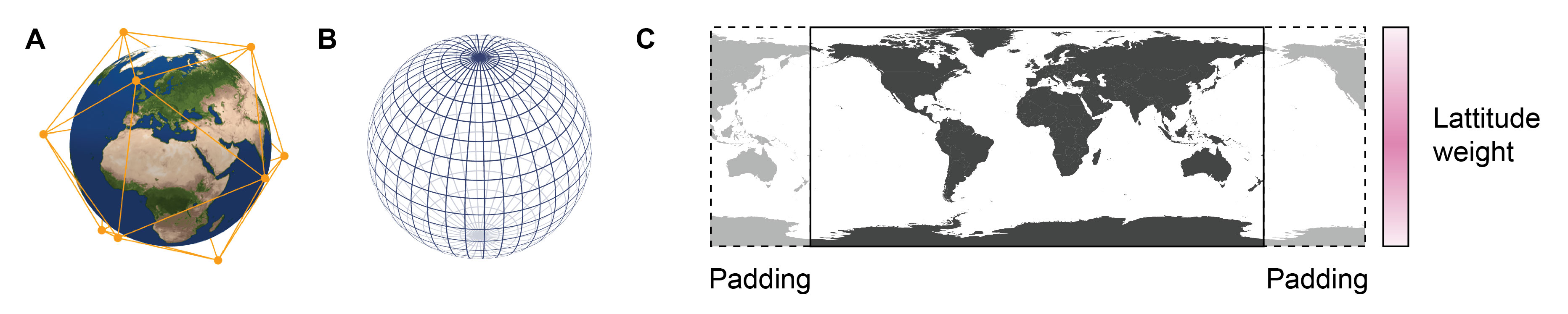Figure 1: Earth representations for weather forecasting. Nodes in triangular graphs (A) encapsulate the earth in a more uniform manner, in contrast to rectangular graphs (B), which are denser at the poles. (C) Earth can be projected on a rectangular 2D grid. Circular padding can be used to account for the continuous longitudinal nature, and latitudinal weighting can be used to de-prioritize the contribution from pole regions. Panel A was taken from Figure 4a of (Adamov and Oskarsson, 2025), which was reused with the permission of the authors. Panel B is under CC BY-SA 3.0 license at Wikimedia Commons, and panel C was adapted from a free image repository.

When considering graph architectures, Joel and Simon found out that flexibility is key, as it provides the model with sufficient capacity to learn. For instance, it is important to include longer edges that can propagate information between distant regions. Interestingly, this performs better than simply increasing the network depth, which also extends the reach of information. There are different hypotheses as to why this might be the case. One possibility is that the ability to transport long-range information already in early layers is beneficial, while deep graph neural networks are known to suffer from message over-smoothing.

Graph capacity can also help mitigate other challenges. Like any architecture, graphs can introduce their own prediction artifacts. For example, the predictions may contain patterns that reflect the underlying structure of the graph mesh. This can be observed as subtle rectangular or honeycomb-like prediction cliffs when using rectangular or triangular graphs, respectively (see Figure 37 of Adamov and Oskarsson, 2025). While there may be ways to fix this by carefully tinkering with the graph structure or operations, much simpler solutions exist in practice. For example, Joel noted that increasing the graph’s capacity (i.e., resolution) while keeping the graph structure unchanged can effectively reduce these artifacts.

Another important factor that should not be overlooked is the computational intensity associated with the chosen graph layout. For instance, Simon and Joel suggested that adjusting the mesh density based on the underlying data resolution could be beneficial. - Regions without fine-grained data could be modeled with a coarser resolution (Figure 2A).

Adjusting the mesh layout based on the underlying data resolution

Typically, the data points are not directly used as graph nodes; instead, they are condensed into a coarser mesh (Figure 2A), which helps to reduce the computational requirements. To enable long-range information propagation, a subset of mesh nodes is selected and equipped with longer edges (Figure 2B), while other nodes focus on fine-grained information.

In regional models, which are described in more detail below, it is common to have regions of interest with high-resolution (local) data, surrounded by boundary regions, where only coarser (global) data is available. In such scenarios, it may be sensible to remove nodes focused on representing fine-grained information from boundary regions, as this information is simply not available (Figure 2A).

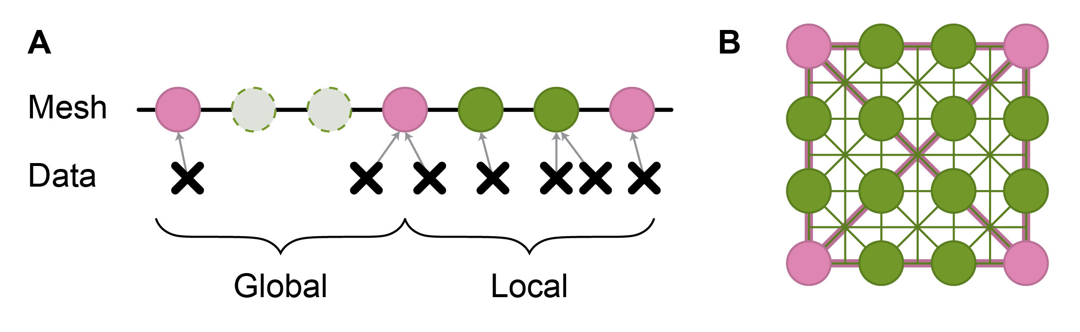Figure 2: The relationship between data points and mesh graph (A) and the mesh graph connectivity (B). In (A), dotted circles represent short-range nodes that may not be needed in the global regions due to sparser data. The illustration of data-mesh connectivity is simplified, with each data point connected to a single mesh node, while in practice, each data point may be connected to multiple neighboring mesh nodes. In (B), a mesh with short-range (green) and long-range (pink) nodes and edges is shown.

Choosing the right data

To make predictions, appropriate input data is, of course, a prerequisite. However, in the machine learning weather forecasting community, models are often trained with input data that is unavailable in the operational setting. For example, training often relies on ERA5, which is a reanalysis dataset. It is heavily preprocessed to increase its physical, spatial, and temporal consistency (Figure 3). ERA5 also utilizes future data to estimate the current atmospheric state, which creates a disconnect with the datasets available in operational context. Besides this, relying on preprocessed data (including operational analysis data; Figure 3) propagates the dependence on classical physics-based systems used for preprocessing.

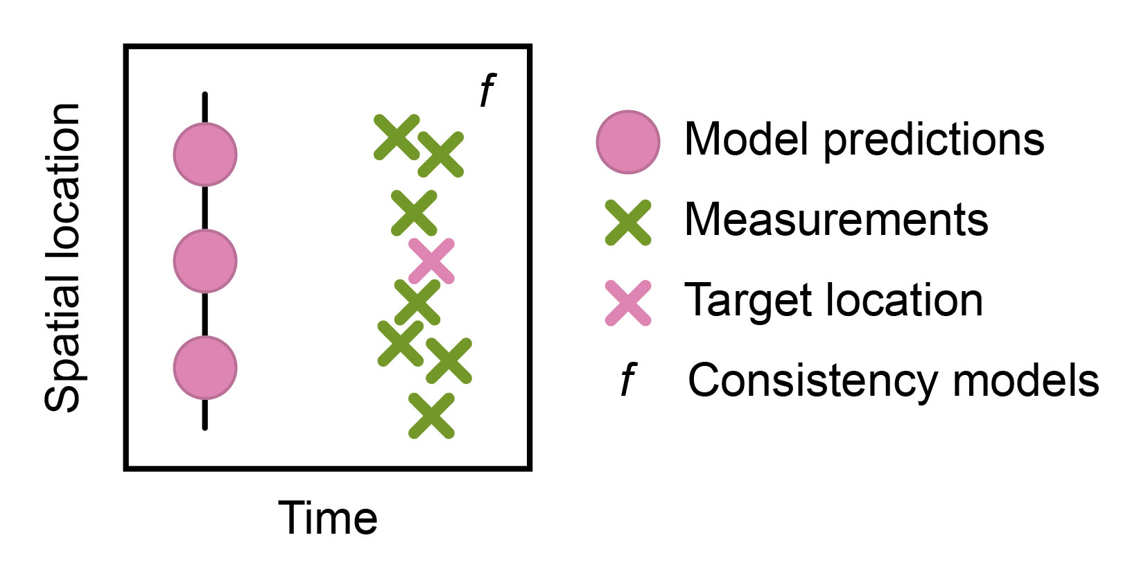Figure 3: Preprocessing used to integrate measurement data into analysis datasets. The data shown in the box is jointly analyzed to predict the best possible estimate of the current weather at the target location (pink “X”). For both operational analysis and reanalysis, the general principles for achieving physically, spatially, and temporally consistent data are similar. However, for reanalysis, data points from a more distant future (e.g., a day) are also used to obtain the estimate of the target time point.

What are ERA5 and operational analysis datasets?

ERA5 is a well-curated historical dataset provided by the European Center for Medium-Range Weather Forecasts (ECMWF). As a reanalysis dataset, ERA5 does not present actual observations; instead, it offers a processed version of the data, ensuring physical, spatial, and temporal consistency. This is achieved by applying equations that govern atmospheric processes, such as fluid dynamics and thermodynamic principles. - Similarly to what is done in classical NWP weather forecasting systems. Moreover, reanalysis outputs for every time-point are influenced by a temporal window around it, effectively creating outputs that have “peeked-into-the future”.

While reanalysis data is not available for operational settings, models often rely on other types of preprocessing (i.e., operational analysis; for a more detailed description of an example operational analysis dataset see this post). These preprocessing pipelines typically combine multiple data sources together with predictions of past atmospheric states to generate a high-quality estimate of the current atmospheric conditions. For example, to estimate temperature at time t and location x , operational analysis integrates temperature measurements from multiple devices (e.g., ground stations or aircrafts) in nearby regions with a prediction from the previous time step (t-1 ).

Thus, while working with ERA5 is convenient for pretraining, it is nevertheless crucial to fine-tune the models on realistic input data at the end³. Moreover, several recent studies have proposed solutions that can directly ingest raw measurements (Alexe, 2024; Allen and Markou, 2025).

When using NWP outputs as the inputs for another model, it is crucial to know how NWP models function. - To obtain clean inputs, it is not enough to simply assess if the NWP outputs are numerically valid (e.g., no missing values). Instead, it is important to understand what these values really represent. An example of this are the border regions in NWP models. They are added to prevent spurious behavior of atmospheric processes when faced with a sharp artificial border. Thus, they do not follow real physical dynamics but rather artificially dampen them (Figure 4).

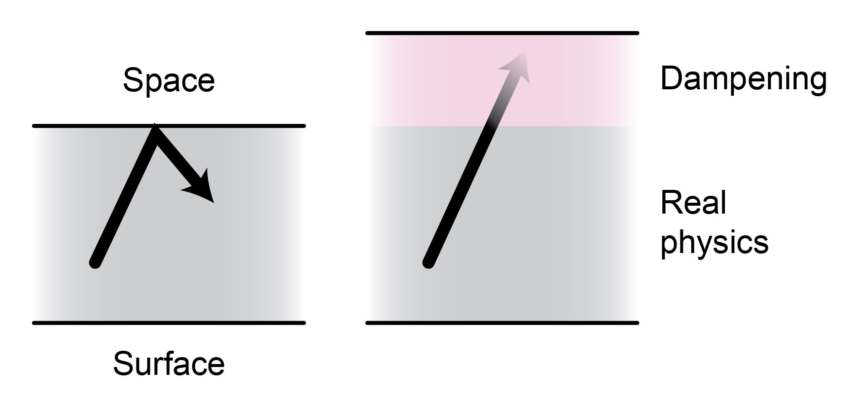Figure 4: Dampening regions in NWP models. They are added at the vertical boundary (right) to prevent spurious dynamics when faced with a sharp border (left).

Artificial boundary regions in NWP models

NWP models use physical laws to simulate the dynamics of the atmosphere. However, unlike the real atmosphere, which transitions smoothly into space, simulations cannot model infinite space and therefore have vertical boundaries. When simulating physical processes, such boundaries can act like a wall, causing reflection. For example, when air waves reach a boundary, they can not propagate beyond it. Since the energy must be conserved, this results in waves bouncing back from the boundary. To prevent such behavior, dampening regions are added. These regions do not adhere to physical laws; instead, they artificially absorb the energy to prevent spurious reflections.

Similarly, embedding a local weather model into the context of a global model is challenging as the two models often differ in how they model atmospheric dynamics, as well as the modeling resolution. To ease this transition, nudging regions are introduced along the lateral edges between the two models. These regions gradually nudge the atmospheric state values of the regional model to align with the values observed in the global model.

While values in these border regions may appear realistic from a numerical perspective, they do not represent valid atmospheric dynamics. Therefore, it is important to exclude data from these regions when training machine-learning models. If this is not done, models may replicate false atmospheric dynamics at the borders.

However, the challenges highlighted above are by no means the only data complications that must be overcome. Sufficient domain knowledge is thus key for correctly utilizing the available data resources.

Common dataset limitations

Simon highlighted some common dataset limitations and biases:

• Many "ML-ready" datasets lack hydrological variables such as sea surface temperature, evaporation, and transpiration. The absence of this information hinders long-term (e.g., sub-seasonal and seasonal) forecasting. - It introduces uncertainty about the full atmospheric dynamics and subsequently leads to less stable autoregressive rollouts.
• In the upper atmosphere, specific humidity values are numerically very low. When converted to relative humidity, this results in abrupt jumps between the values 0% and 100%. Unfortunately, many datasets provide only relative humidity, which complicates model training due to its instability.
• The atmospheric values are often only coarsely resolved across the vertical axis due to computational constraints.
• Individual NWP models, which are involved in the generation of input data, frequently exhibit biases of their own. However, these are often not well-known in the broader community and therefore not properly accounted for.

Which atmospheric processes must be accounted for?

Furthermore, it is crucial to decide in advance what the model may be used for and thus should be able to predict. For example, while most models tend to focus on near-surface variables (i.e., troposphere), the importance of higher atmospheric levels (i.e., stratosphere) should not be overlooked. Simon pointed out that the aerospace industry is an important client of MeteoSwiss, requiring accurate forecasts not just near the ground but also higher up in the atmosphere. Moreover, recent research suggests that including the stratosphere improves long-range weather predictions (i.e., spanning several weeks) and enhances climate studies (i.e., over years or decades). This underscores the value of considering how the stratosphere can be effectively integrated into future weather models.

However, modeling the stratosphere requires stratospheric data, which can not be handled in the same way as data from the lower troposphere. For example, the commonly used operational analysis data is often unreliable in the stratosphere. Thus, it is important to include additional data sources, such as raw satellite observations.

Evaluation that will be trusted by the community

For a model to gain recognition of the weather forecasting community, it is not enough to achieve good scores on standard benchmarks. Namely, low mean squared error (MSE) on the ERA5 data - often dubbed the “ImageNet” for weather - is not convincing on its own. Therefore, Joel and Simon listed multiple evaluation approaches that increase model credibility:

• Qualitative evaluation: Beyond reporting aggregated metrics (e.g., average MSE), it is important to examine individual model predictions. By doing so, we can spot important biases that might be hidden when everything is averaged together.
• Physical consistency: Rather than only checking how close the predictions match the ground truth, it can be more meaningful to determine whether predictions adhere to physical principles. For example, this may include assessing whether surface pressure remains consistent across forecast days or whether moisture is conserved across vertical atmospheric layers⁴. However, Simon noted that setting up such an evaluation may be more challenging, especially for limited-area models.
• Spatial consistency: Given that weather phenomena are characterized by moving shapes (e.g., clouds), it is important to evaluate the shape of the predictions and not only their point-wise values. For instance, the SAL precipitation score (Figure 5) evaluates whether precipitation patterns are realistic (e.g., not too spiked). Moreover, it distinguishes between errors in amplitude and location. For example, if a storm is spatially displaced, the MSE would impose a penalty equal to the full amplitude for both the area where the storm was predicted but did not occur (false positive) and where it did occur but was not predicted (false negative). In contrast, SAL would report an error only for the location, but not for the amplitude.
• Weather warnings: Because weather forecasts are used to issue weather warnings, it is important to evaluate how often the model would lead to wrong warning decisions. Such evaluations are usually threshold-based, determining whether a certain weather event meets the criteria for a specific warning category.
• Observation data: Although observation data is sparse and can be affected by measurement errors, it is indispensable for evaluation. Namely, the evaluation based solely on analysis or reanalysis data has major limitations. As this data consists of model-corrected observations, models that operate in similar ways or have similar biases will be erroneously favored. Moreover, such data is often unnaturally smoothed, missing local extremes and surface-related effects (e.g., variation in heat capacity). Thus, observation-based evaluation is key for achieving realistic and locally relevant predictions.
• Case studies: It is common to test the model’s ability to predict selected historical weather events, particularly extreme occurrences such as hurricanes. These case studies evaluate the model from multiple perspectives, such as consistency of weather dynamics, adherence to physical principles, and ability to model extremes.

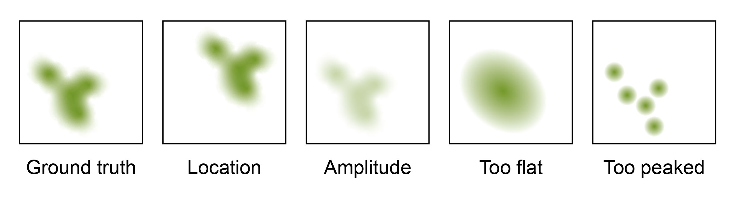Figure 5: SAL precipitation score, which evaluates structure, amplitude, and location. Shown are different types of errors within individual SAL categories.

Laying the deterministic objective to rest

Weather forecasting models are often trained with a simple deterministic objective - given the current atmospheric state, predict the subsequent state. However, this approach tends to produce overly smooth predictions. For example, if the model predicts an extreme weather event, such as a thunderstorm, but with a shifted location, it is penalized twice - once for missing the actual event (false negative) and again for the false positive on the shifted location. Thus, the model learns to cheat by avoiding predicting extreme events and rather sticks to the mean (Figure 6). This is further aggravated when combined with an L2 loss (e.g., MSE), which heavily penalizes false positive predictions of extreme events⁵.

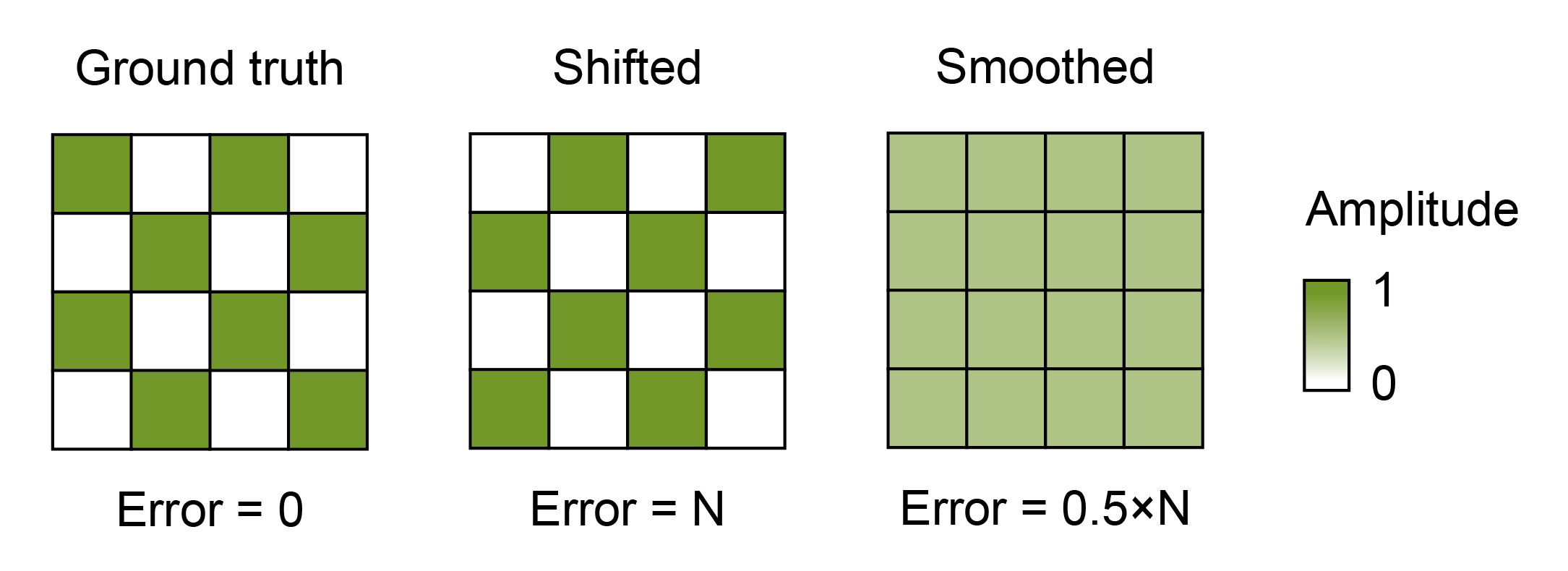Figure 6: Bias towards smooth predictions. Due to the double penalty faced by shifted predictions with true amplitude, smoothed predictions are preferred.

This over-smoothing also negatively affects autoregressive rollouts. - With each autoregressive step, errors accumulate, severely degrading the performance. While this is a common issue in all autoregressive models, such as those used in natural language processing, Shoaib explained that it is especially problematic in weather forecasting. While models with discrete outputs (i.e., tokens) have the chance to output the exact correct token, this is almost impossible for models with continuous outputs (Figure 7). Thus, it is much harder to manage error accumulation.

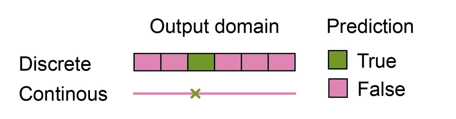Figure 7: The chance of making an error-free prediction is much lower in models with continuous rather than discrete output. Even when continuous output models make relatively small errors, these errors accumulate across autoregressive steps.

Mitigating compounding errors

In practice, compounding errors are often mitigated by fine-tuning the models on autoregressive rollouts. This helps the model to learn how to produce high-quality predictions even when using its own noisy predictions of earlier steps as input. While this technique has long been used to mitigate error accumulation in other fields, such as reinforcement learning (Ross, 2011), Shoaib pointed out that it has only recently become popular in the weather community.

Recent research has shown that probabilistic objectives⁶, such as those used in diffusion models, produce sharper predictions than deterministic objectives (Price, Sanchez-Gonzalez, Alet, and Andersson, 2024). The increased sharpness also helps improve autoregressive performance, since it reduces error accumulation across iterations.

Individual probabilistic predictions stay sharp since each prediction does not need to capture the full range of possible future outcomes by itself (Figure 8). Namely, the model outputs multiple potential predictions of the future, and together these predictions form a distribution that reflects the uncertainty about the future. In contrast, individual deterministic predictions are designed to represent the mean of the distribution across possible future states (Figure 8).

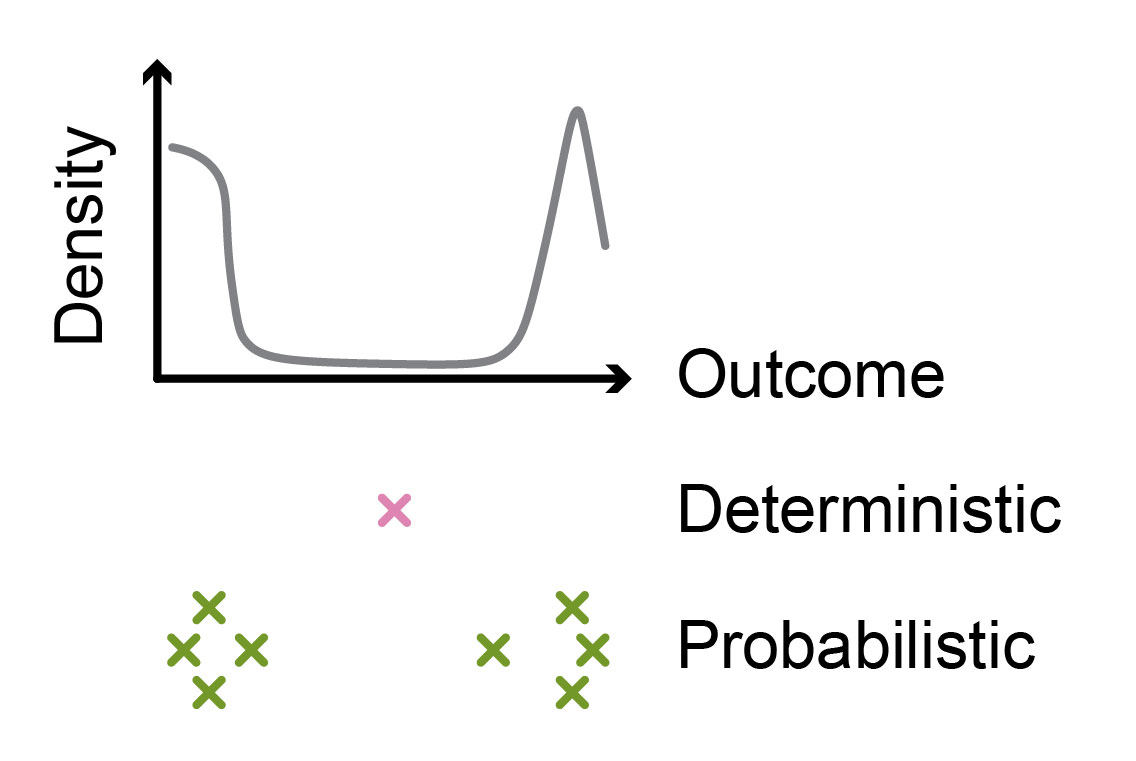Figure 8: Predictions of models with probabilistic objectives are not smoothed towards the mean of the training outcome distribution. Similar input conditions (e.g., similar atmospheric states from different time points, such as days or years, or locations) may result in different weather outcomes (top). A deterministic model with MSE loss would predict the mean of the training outcomes (middle). The predictions of the probabilistic model would be more realistic, resembling the samples from the real outcome distribution, with their distribution following the training data outcome distribution (bottom).

Iterative prediction refinement in diffusion models

Another advantage of diffusion models is their multi-step prediction process, as opposed to generating outputs in a single step from the input. The model first generates an approximate prediction that still contains substantial noise. Through subsequent steps, the model refines this prediction by gradually removing the noise. This allows the model to progressively build up the details.

Despite their advantages, diffusion models have not yet been widely adopted in the research community. The main barrier is the high computational resource demand, both for training and inference. While such demands do not necessarily prohibit operational use, they make it much harder for researchers to explore new modeling ideas.

Predicting at high resolution

Models that forecast at high spatial and temporal resolution are often designed for specific regions of the Earth. This is partly because creating detailed forecasts requires a lot of computational resources, and partly because these models rely on additional data that is only available for limited areas.

Types of local prediction approaches

To forecast regional weather at higher resolution, different methods were proposed. Many earlier NWP approaches subsequently inspired neural network techniques, which now fall into the three main categories listed below. While all three have resulted in strong-performing models, Joel pointed out that it is still uncertain which one will become standard in the operational setting (Wijnands, Van Ginderachter, François, and Van den Bleeken, 2025).

• Downscaling takes as input a coarse global forecast for a specific time point and region and outputs a higher-resolution prediction (Mardani, Brenowitz, and Cohen, 2025).
• Forecasting with boundary forcing uses global weather information around the target region (i.e., the border), which spans a window of both past and future border states, to forecast regional weather (Oskarsson, 2023). This approach can also be combined with downscaling (Adamov and Oskarsson, 2025).
• Forecasting with stretch-grid approaches models global weather, but uses higher spatial resolution at the target region (Nipen, Haugen, Ingstad, Nordhagen, Salihi, Tedesco, and Seierstad, 2024).

One promising direction, highlighted by Simon and Joel’s research, is the integration of downscaling (i.e., increasing resolution) and forecasting (i.e, predicting new weather states), (see box Types of local prediction approaches). The ability to combine the two is unique to machine-learning models, as the traditional approaches were limited to either forecasting (NWP models) or downscaling (statistical methods).

Nevertheless, in their paper, they faced challenges when integrating downscaling and boundary-forcing-based forecasting. In some situations, the models would switch between downscaling using time-matched global data, and forecasting for time-steps without global data. This resulted in inconsistent behavior that varied depending on the available information. Ideally, all global information should be integrated to create global representations that subsequently inform local predictions. During our conversation, Joel and Simon hypothesized about strategies that could lead to more consistent behavior:

• Two-stage training: The model could initially be trained to forecast without overlapping global information. Subsequently, the model could be fine-tuned⁷ to take advantage of the overlapping information and thus further refine its internal representations of the global state.
• Masking of overlapping global information: The global data overlapping the target region could be partially masked, so that the model can not rely entirely on downscaling.

In search of data for building forecasting models

Despite the ongoing collection of weather data all across the globe, gaining access to climate datasets can still be surprisingly challenging. Many of the datasets are not openly available; instead, they belong to individual states. Thus, special requests are needed to access them.

In addition, the lack of centralized data collection makes it difficult to integrate datasets from various sources. Challenges range from data transfer to dataset-specific cleaning, converting them into a common format, and mitigating dataset-specific biases. The ingestion of diverse datasets often involves complex workflows, which increases the chance of introducing errors (e.g., non-numerical values - nan) and complicates tracking thereof.

In response to these challenges, a variety of centralized data access initiatives have been established, ranging from international (e.g., The European Weather Cloud) to research institution-specific collections. There have also been attempts to standardize data formats, such as the GRIB2 schema. However, even within this schema, authors commonly lean towards individual interpretations of the common definitions, leading to discrepancies.

Common research tools

Apart from data availability, Shoaib, Simon, and Joel emphasized the importance of computational tools for their research. For example, they highlighted xarray and zarr for handling large annotated datasets, wandb for benchmarking infrastructure, and scores and WeatherBench for efficient large-scale evaluation. Moreover, foundation model initiatives, such as Aurora (Bodnar, Bruinsma, Lucic, Stanley, Allen, 2025) and WeatherGenerator, are expected to influence future weather modeling.

Other researchers from diverse domains, who participated in previous blog posts, have similarly emphasized the importance of tools for handling large-scale annotated data and for tracking computational experiments. This indicates a read thread among valuable research tools.

Key takeaways

To facilitate the integration of neural-network-based forecasting methods into the operational setting, the research community is actively exploring the predictive and computational performance of various approaches. An important takeaway is that relatively simple architectures can be effective, provided the model is supplied with relevant data and sufficient capacity. However, access to required datasets remains challenging, which hinders the development of realistic models and trustworthy evaluation.

References

• Adamov and Oskarsson, et al. Building Machine Learning Limited Area Models: Kilometer-Scale Weather Forecasting in Realistic Settings. arXiv (2025).
• Alexe, et al. GraphDOP: Towards skillful data-driven medium-range weather forecasts learnt and initialized directly from observations. arXiv (2024).
• Allen and Markou, et al. End-to-end data-driven weather prediction. Nature (2025).
• Bodnar, Bruinsma, Lucic, Stanley, and Allen, et al. A foundation model for the Earth system. Nature (2025).
• Dunstan, Strickson, Bennett, Bowyer, Burnand, Chappell, Coca-Castro, Dale, Daub, Eftekhari, Janmaijaya, Lillis, Salvador-Jasin, Simpson, Chan, Elmasri, France, and Madge, et al. FastNet: Improving the physical consistency of machine-learning weather prediction models through loss function design. arXiv (2025).
• Holmberg, et al. Accurate Mediterranean Sea forecasting via graph-based deep learning. arXiv (2025).
• Mardani, Brenowitz, and Cohen, et al. Residual corrective diffusion modeling for km-scale atmospheric downscaling. Communications Earth & Environment (2025).
• Nipen, Haugen, Ingstad, Nordhagen, Salihi, Tedesco, and Seierstad, et al. Regional data-driven weather modeling with a global stretched-grid. arXiv (2024).
• Oskarsson, et al. Graph-based neural weather prediction for limited area modeling. NeurIPS Workshop on Tackling Climate Change with Machine Learning (2023).
• Price, Sanchez-Gonzalez, Alet, and Andersson, et al. Probabilistic weather forecasting with machine learning. Nature (2024).
• Ross, et al. A Reduction of Imitation Learning and Structured Prediction to No-Regret Online Learning. AISTATS (2011).
• Siddiqui, et al. Exploring the design space of deep-learning-based weather forecasting systems. arXiv (2024).
• Watt-Meyer, et al. ACE2: accurately learning subseasonal to decadal atmospheric variability and forced responses. npj Climate and Atmospheric Science (2025).
• Wijnands, Van Ginderachter, François, and Van den Bleeken, et al. A comparison of stretched-grid and limited-area modelling for data-driven regional weather forecasting. arXiv (2025).

Footnotes

1. The post was not yet proofed by Shoaib, so the content may be biased towards my personal interpretation of our discussion. ↩︎ ↩︎²

2. Image-focused architectures require data to be organized into a regular grid, where all vectors along a given dimension have the same number of elements. In contrast, graph architectures can operate on non-regular grids. A common example is the reduced Gaussian grid, which has a decreasing number of longitude nodes towards the poles. Moreover, different grid resolutions may be chosen across spatial regions, such as a coarser global and a finer-grained regional resolution (Adamov and Oskarsson, 2025). ↩︎

3. Different data sources can be used to replace ERA5 in the operational setting. For example, operational analysis data can be used for initial conditions. In the case of regional models, real forecasts can be used for boundary forcing. ↩︎

4. To make sure that models adhere to these laws, they can also be directly enforced upon prediction as hard constraints (Watt-Meyer, 2025) or integrated as soft constraints within the loss function. ↩︎

5. Some studies have explored alternative losses instead of the MSE loss to reduce prediction smoothing (Dunstan, 2025). ↩︎

6. It is important to distinguish between probabilistic predictions and probabilistic objectives. Probabilistic predictions can be obtained in different ways. One common approach is to combine deterministic models, where each model produces a single output, into an ensemble. Alternatively, input data can be perturbed with noise to yield different outputs from a single model. Recently, models with probabilistic objectives (e.g., diffusion models) were proposed. These models predict a whole distribution of possible weather outcomes, meaning they can inherently produce a variety of outputs for a given input. ↩︎

7. Recent studies have demonstrated the benefit of fine-tuning foundation weather models for specific tasks, for which only limited data is available, such as high-resolution prediction (Bodnar, Bruinsma, Lucic, Stanley, Allen, 2025). ↩︎