Finding a match between genomics and machine learning

Expand all detail boxes for printing

Statistics is the cornerstone of genomics. - Nevertheless, can other approaches also yield meaningful genomic insights?

Genomics is a challenging field for method development. - The sample sizes are often small, and results must be both interpretable and highly trustworthy. Thus, classical statistical methods are still the gold standard. In discussions with Boyang, Alan, and Yasha, we explored where other computational approaches, such as machine learning and new algebraic algorithms, can support genomics research.

Overview of the discussed publications

Boyang developed a method for discovering interactions between genetic variants (i.e., epistasis) that provides greater statistical power and scales better to large datasets (Fu, 2025). The test builds upon the standard regression framework, while the solution to the regression equation is sped up via randomized linear algebra.

Alan constructed a scalable model that helps increase the power of genetic association studies (Amin and Potapczynski, 2025). It provides a meaningful prior for the probability of each variant being associated with a phenotype. This prior is derived from auxiliary genomic information.

Yasha proposed a new protein sequence model for phylogeny reconstruction. It can speed up classical phylogenetic workflow and may, in the future, improve protein property prediction (Ektefaie and Shen, 2025). This is achieved by training the model on the evolutionary relationships of multiple protein sequences.

This blog post highlights topics that got less focus in the publications. If you are more generally interested in the design of models for genetic data, I recommend reading the original papers, as many topics are skipped here. Furthermore, this post does not aim to provide a comprehensive overview of the field; instead, it focuses on highlights from our conversations.

While this blog post is based on discussions with Boyang, Yasha, and Alan, I often omit their names for the sake of readability.

Sections list

• A brief methodological introduction
  • Detecting genetic-phenotype associations
    • Increasing power with a prior based on genetic context
    • Efficiently detecting epistasis
  • Protein embeddings for phylogenetic tree reconstruction
• Is machine learning trustworthy enough?
  • Going beyond the "default" methods
  • Finding new data to improve performance
  • Let the data speak
• Answering genomics questions with limited compute resources
  • How flexible does the model need to be?
  • Overcoming resource constraints

A brief methodological introduction

The summaries below provide a quick and simplified¹ methodological background for the topics discussed in this post.

Detecting genetic-phenotype associations

To determine which genetic variants (e.g., changes in DNA) are associated with a specific phenotype (e.g., disease), the following regression model is commonly employed in what are known as genome-wide association studies (GWAS):

\[y = C\alpha + X\beta + \epsilon\]

where $y$ is the phenotype, $C$ are known covariates to be adjusted for (e.g., age, sex), which are of shape $N \times K$ with $N$ individuals and $K$ covariates, $\alpha$ are the corresponding effect sizes (e.g., how much does each covariate contribute to the phenotype), $X$ is the genotype matrix of shape $N \times M$ with $M$ genetic variants, $\beta$ are the corresponding effect sizes of the variants, and $\epsilon$ is independently and identically distributed (IID) noise.

As the number of subjects is commonly smaller than the number of genetic variants ($N << M$), the above linear system is underdetermined. Thus, $\beta$ must be constrained. This is commonly done by assuming that all $\beta$ coefficients are sampled from a normal distribution:

\[\beta_{m} \sim N(0,\frac{\sigma^{2}_{g}}{M})\]

where $\beta_{m}$ corresponds to individual genetic variant $m$ and $\sigma^{2}_{g}$ is total genetic variance, normalized via $M$ to model per-variant variance.

This is known as the “infinitesimal” model. It is biologically well-motivated: many phenotypic traits are shaped by a large number of genetic variants, each contributing only a small (infinitesimal) effect (Barton, 2017).

Increasing power with a prior based on genetic context

However, the large number of genetic variants reduces the power to detect genetic-phenotype associations after multiple testing correction². Thus, a prior based on the genetic context can be used to allow for a larger absolute value of $\beta_{m}$ for variants that are generally more likely to be causal (i.e., lead to a specific phenotype), thereby increasing power (Figure 1). For example, variants that affect protein function or gene expression are more likely to be causal.

To obtain this prior, a model that predicts $\sigma^{2}_{g,m}$ based on local genetic sequence can be constructed. In practice, the model can be fit using pre-computed effect sizes and trained on all but one chromosome. Subsequently, it can be used as a prior to the above regression equation on the left-out chromosome.

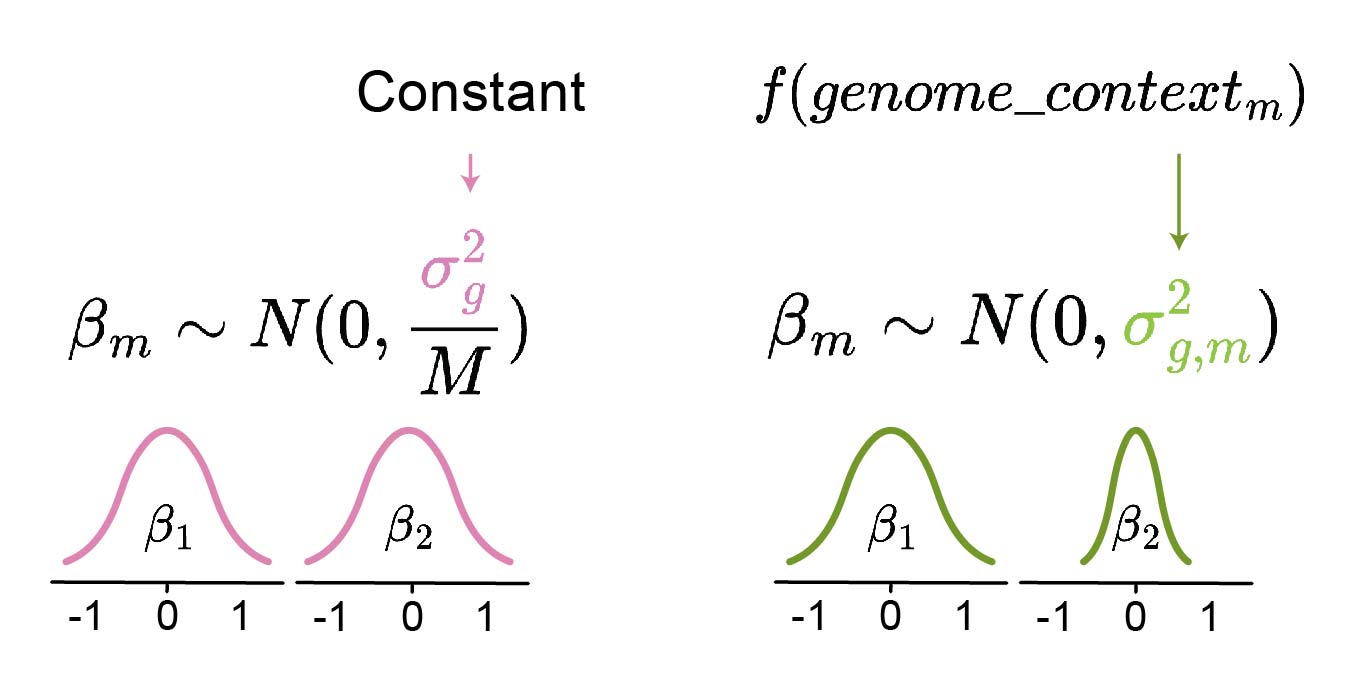Figure 1: Comparison of different approaches for constructing the β sampling distribution. Instead of using a constant σ²_g for all variants m (left), σ²_g,m can be inferred for each variant individually based on its genomic context (right). The prior model f predicts whether the variant is unlikely to be causal (low predicted variance σ²_g,m of β_m sampling distribution, e.g. β₂) or not (high variance, e.g. β₁). The latter produces a wider prior distribution and thus allows the downstream statistical model to decide upon the size of β_m (either small or large absolute value). Thus, the prior prediction model can also account for its own uncertainty by outputting high variance.

Alan and his colleagues improved upon this framework in their model DeepWAS (Deep Genome-Wide Association Studies), with two main contributions:

• They used a more flexible prior model, specifically a transformer with a large number of genetic features, rather than a simple linear model based on only a few features. Moreover, they demonstrated that large models can be successfully fit if leveraging all available data, including information about the linkage-disequilibrium³ (LD) induced dependence between $\beta_{m}$. This information was omitted or simplified in previous works due to computational complexity, resulting in lower power and less accurate predictions.
• They were able to fit the full likelihood of the $\beta_{m}$ sampling distribution, including the LD structure, by using fast linear algebra methods.

Efficiently detecting epistasis

Epistasis is a non-additive (i.e., multiplicative) interaction between multiple genetic variants that collectively affect the phenotype. Its detection is challenging, due to both low power and high computational requirements.

To detect pairwise epistasis, $\frac{M \times M - 1}{2}$ associations need to be tested. The complexity increases further when considering higher-order interactions (i.e., triplets, quadruplets, and so on). To overcome the multiple-testing burden, “marginal” epistasis can be tested. - Instead of testing the epistasis between pairs of variants, each variant can be tested for interactions with the whole genetic background at once (Figure 2). The following extension of the above-described regression model can be employed to test the marginal epistasis of an individual variant $m$:

\[y = C\alpha + X\beta + E_{m}\gamma_{m}+ \epsilon\] \[\gamma_{m} \sim N(0,\frac{\sigma^{2}_{gg,m}}{M-1})\]

where $E_{m}$ represents interactions between variant $m$ and other variants, being a matrix of shape $N \times (M-1)$ obtained as $E_{m} = X_{m} \odot X_{-m}$ with $X_{m}$ being the $m$-th column of matrix $X$ and $X_{-m}$ being the matrix $X$ without the $m$-th column. The significance of marginal epistasis is assessed using a variance-component model. It assesses whether the variance $\sigma^{2}_{gg,m}$ , which describes the distribution of epistatic effects of variant $m$ with other variants, is above zero. Thus, for each variant, a single statistical test is performed, rather than one test per interaction (e.g., $M-1$ tests), resulting in increased power.

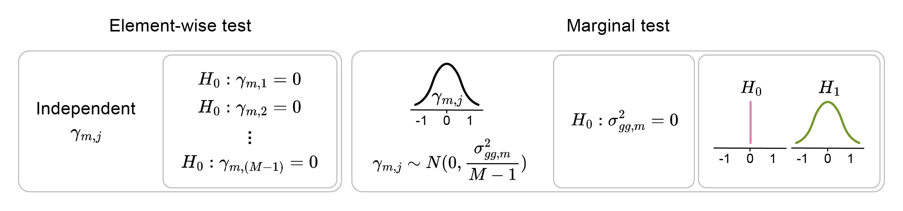Figure 2: The marginal interaction test evaluates interactions with any of the elements rather than with each element individually. The null hypothesis assumes there are no interactions between element m and other M-1 elements j.

Solving this equation requires multiplication of large matrices (i.e., $X$ and $E$). To speed this up, Boyang employed a randomized linear-algebra technique similar to sketching. Sketching projects high-dimensional matrices into lower dimensions using a random lower-dimensional projection matrix $U$, obtaining a projection $UX$, where $dim(U) = R \times N$ with $R << N$. When the dimensionality ($R$) of the random projection matrix is high enough, the compressed matrix representation is sufficiently accurate for downstream linear algebra applications. This approach distinguishes FAME (FAst Marginal Epistasis test) from other marginal epistasis tests.

Protein embeddings for phylogenetic tree reconstruction

Phylogenetic trees aim to model evolutionary relationships between organisms. Methods for tree reconstruction often require substantial computational resources because the space of possible trees grows rapidly with the number of species. Briefly, they first compare biological sequences (e.g., DNA or proteins) across species, identifying optimal sequence alignments (i.e., multiple sequence alignments, MSAs). Based on MSA, they infer species-relatedness, accounting for the probability that individual sequence differences arise during evolution. Finally, they fit a tree that best captures the relationships among all the species. Fitting the tree is complicated, as it requires inferring the optimal order of consecutive mutation events that led from an unobserved shared ancestor to the development of the analyzed species.

Yasha and his colleagues proposed a faster approximation, which uses a simple neighbour-joining algorithm on distances between protein embeddings to reconstruct the tree. To make this possible, the protein embeddings need to be generated by a dedicated model that captures evolutionary relationships. Thus, their embedding model, Phyla, is not trained on the standard sequence reconstruction (e.g., masked language modeling or autoregressive loss) but rather to generate embeddings whose distances correspond to evolutionary relationships⁴ (i.e., contrastive learning, Figure 3). To provide an evolutionary context for the embedding, multiple sequences are embedded simultaneously.

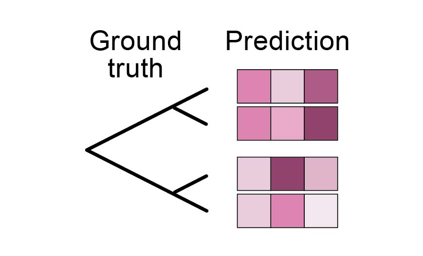Figure 3: Phylogenetic reconstruction objective. It evaluates whether the distances between predicted sequence embeddings match the ground-truth phylogenetic tree.

Future Phyla applications

Yasha mentioned that they are currently actively investigating different Phyla extensions and applications. One of the topics he highlighted was sequence comparison. - While many models rely on pre-computed MSA (e.g., for protein structure prediction), the MSA computation is time-consuming. Thus, Phyla could be fine-tuned to provide sequence representations that could substitute the MSA. Similarly, Phyla could be fine-tuned to generate adaptive sequence comparisons, in which the importance of individual sequence differences (i.e., changes at specific positions) could be tailored to the task, unlike in classical MSA.

Is machine learning trustworthy enough?

While many application domains have been revolutionized by machine learning (ML), the state-of-the-art genomic methods still often rely on classical statistical methods. This may seem like the perfect opportunity for new method development, Boyang noted; however, there are good reasons behind the lack of ML methods. Despite various ML methods having been developed (Dibaeinia, 2025), they are not widely used as they often lag behind classical approaches. In line with this, Alan observed a widespread lack of trust in newly developed ML models.

In GWAS, results directly influence research activities (e.g., the generated hypotheses guide new experiments). Thus, there is a need for well-calibrated and trustworthy results. While ML methods, such as random forest, provide high-quality predictions, their interpretations are often less reliable. However, it is the interpretation (i.e., which features are associated with phenotypic outcome) rather than the predictive performance (i.e., which phenotype is expected based on the specific feature values) that is of primary interest⁵.

Boyang illustrated it as follows: Given two correlated predictive features, $A$ and $B$, a random forest model can choose either for high-quality predictions. There is no guarantee that it will be possible to determine the causal role of the two features based on the model’s decision rules. Moreover, if the LD-based variant correlation structure is not accounted for, non-causal variants located near causal variants may also strongly contribute to the prediction.

However, Alan pointed out a common misconception: that more powerful models are less reliable for feature importance analysis. It has been shown before that models with the lowest false discovery rate also have high power (Tansey, 2021). This can be explained by model misspecification: If the model is unable to capture real relationships between the target and the explanatory variables (i.e., due to not being able to consider interactions, etc.), the feature importance will be wrongly attributed to the available features (Huggins, 2023; Zhang, 2022). Thus, whether using a flexible deep learning model or a statistical test, it is important to set it up with potential confounding in mind and to be aware of how its guarantees should be interpreted.

Another common critique of deep learning models is that their flexibility makes them more likely to overfit to spurious correlations. For example, living in a highly polluted area can be a phenotypic confounder for disease onset, similar to smoking. At the same time, individuals living in this area may accumulate similar genetic variants, even though these variants do not directly cause the specific disease. If the relevant environmental covariates are unknown, it may seem like these genetic variants are associated with the disease (Figure 4). While, in fact, the effect should be attributed to the environment, not to accumulated genetic variation. This is a problem for both classical and deep learning approaches. However, if the population genetic structure is complex, as is expected, its effect may be less likely to be picked up by a lower-capacity model than, for example, a transformer. Is this likely? Hard to say, said Alan. - Nevertheless, it is a common concern in the community. Thus, he highlighted the importance of careful model validation, as explained below.

Figure 4: Confounding by population structure. If the environment is causing both a specific phenotype and the accumulation of specific genetic variants, the correlation between the phenotype and genotype may be misinterpreted as causal.

How to validate that a model is picking up causal effects?

A common strategy to test whether a polygenic risk score (PRS; the predictor of phenotype based on genotype) is based on true genetic signals (i.e., variants directly influencing the phenotype) or confounding environmental factors (i.e., genetic population structure) is to use mother-father-child trios (Morris, 2020). For example, a pre-trained PRS can be tested on an independent trio cohort by comparing the child’s PRS predictions with those from an artificially constructed genotype comprising variants the child did not inherit from its parents. If the two are equally predictive of the child’s phenotype, that indicates that the PRS relies on confounding genetic variants.

However, as trio data has more limited availability (e.g., it is more often behind a paywall and has a smaller size), Alan used another approach. He trained the model, which predicts whether variants are likely to have phenotypic effects based on genomic context, on some chromosomes and tested it on held-out chromosomes. This confirmed that his model is learning true relationships between the variant causality and the neighboring genomic architecture, rather than simply memorizing genomic patterns around specific training variants.

Besides this, he also highlighted a more generally applicable method (Candès, 2018) that allows for testing whether the model is learning real phenotype-genotype relationships or simply memorizing population structure. The core idea is to construct knockoff features $\tilde{X_{i}}$ that are conditioned on the rest of the features $X_{-i}$ independent of the outcome $Y$. Namely, $\tilde{X_{i}}$ is randomly sampled conditioned on $X_{-i}$, leading to conditional independence to $Y$. Thus, the population structure within $\tilde{X}$ is preserved, but the relationship with $Y$ is perturbed. This allows testing whether the knockoffs are less predictive of $Y$ than the real variables, meaning that the real variables $X$ carry genuine predictive signals beyond the shared population structure.

GWAS data is also often believed to be too small to reliably fit more flexible ML models. The number of samples is usually much smaller than the number of tested genetic associations. When used directly in ML models, this can lead to poor performance because the models are underdetermined. However, Alan showed that there is enough data for high-quality model fits. - The key was to use all of the available information, including the computationally-intensive LD structure (Figure 5).

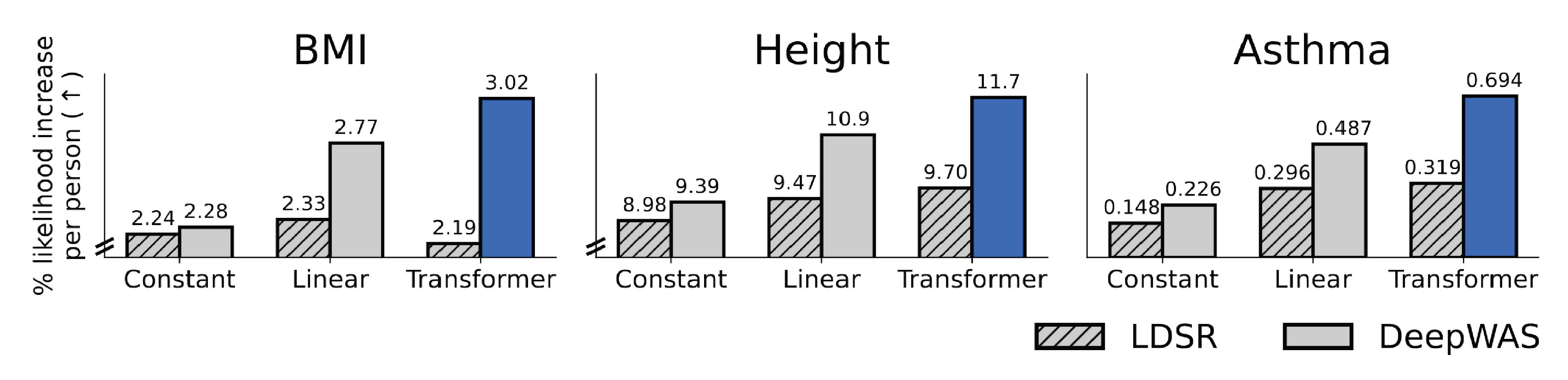Figure 5: Improved performance by combining flexible models and all available information. The plots show model performance (y-axis) with different priors for variant effects (x-axis; i.e., a constant prior across all genomic positions or a prior based on genomic context predicted with a linear or transformer model). When using all available information (i.e., including dependencies among the effects of individual genetic variants), the larger transformer model (DeepWAS) outperformed simpler models (e.g., a linear model). This is not the case when this information is not used (LDSR), in which case the more flexible model can even degrade performance. The image was adapted from Figures 4 and 5 of (Amin and Potapczynski, 2025), which is published under CC BY 4.0 license on Open Review.

With all this in mind, before introducing a new ML model, one should carefully examine which model guarantees are required to make the results useful in practice. Moreover, for ML models to be useful, they do not need to replace statistical methods one-to-one. Instead, progress can stem from finding ways in which the two complement each other. For example, Alan’s two-stage approach, in which the predictive performance of an ML model is used to construct a high-quality prior, which is subsequently employed in a regression-based test, is a good example.

Deciphering the meaning of biological interactions

Another area where ML may benefit genetic studies is supporting the interpretation of phenotypic associations. Individual GWAS studies often generate dozens of potential associations, which require careful interpretation to design future experiments. This often requires extensive manual research, examining existing literature to prioritize potential associations between genetic positions and biochemical disease mechanisms.

Boyang mentioned that large language models turned out to be genuinely useful for this task and are routinely used in their group. He finds them especially helpful for evidence gathering, such as finding biochemical mechanisms that could link the variant to the disease. Before, one would need to use tools like FUMA to explore questions such as: Has the variant been associated with changes in gene expression before? In which cells is the gene that contains the variant expressed? Is the variant located within genomic regions involved in gene expression regulation? After some interesting evidence was found, this needed to be confirmed by digging through a heap of papers.

In contrast, with LLMs and agentic tools, it is possible to start from a hypothesis and ask a more direct question. For example, if one finds a variant related to both liver disease and Alzheimer’s disease, one can directly ask whether there is any literature connecting the two through shared regulatory or metabolic pathways. Boyang highlighted that the LLMs agents are very good at quickly surfacing relevant studies and making cross-domain connections that would otherwise take a lot of time.

However, he also highlighted that they don’t replace careful human judgment. - The researcher still needs to verify the evidence and be cautious about over-interpreting causal claims. Thus, agentic-driven interpretation should not be regarded as a completely autonomous process.

Going beyond the “default” methods

Yasha speculated that the underperformance of ML methods may also be explained by how they are applied to genomics tasks. Most commonly, architectures are taken directly from other domains, such as language and image processing, and forced upon biological data. However, there is a lack of modeling approaches tailored to individual biological data types. He speculated that future architectural developments may open up new ML use cases in genomics.

When Yasha started developing Phyla, he first combined the evolutionary objective with a standard unsupervised pretraining objective - the masked language modelling (MLM) loss. However, he later realised that the two losses actually compete against each other. In fact, when the MLM loss was active, the model was unable to learn to generate embeddings that encode evolutionary relationships between sequences.

This is an interesting observation, as one might expect that objectives for sequence reconstruction (i.e., filling in the blanks given a sequence context) and sequence comparison (i.e., generating representations that reflect similarity) would be complementary. As this is not the case, it may be worth reconsidering many of the current protein analysis workflows that are primarily based on MLM loss. For example, is protein property prediction, a common application of embeddings from MLM-based models, more in line with reconstruction or rather with the comparison objective (Figure 6)?

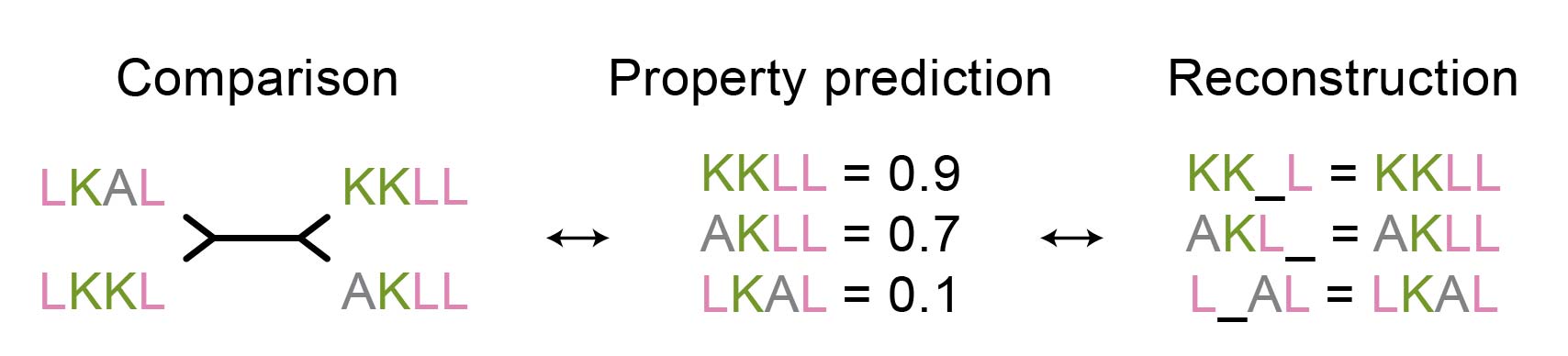Figure 6: Is the property prediction task closer to comparison or reconstruction pre-training objective?

Yasha suspects that it may be the latter (Figure 7). His initial motivation for the new model was to improve the generalisation ability of protein sequence models. Instance comparison is a task that requires stronger reasoning capabilities than reconstruction, thus also leading to better generalisation, Yasha explained. Namely, if the model learns to evaluate differences between sequences, this skill is more transferable to completely new sequences than filling in the blanks in sequences, which relies on memorising training-set patterns. A similar pre-training objective may also be beneficial in other fields where relationships between instances are naturally present, such as for cells within tissue.

The difference between positive/negative and tree contrastive loss

Despite the tree-based quartet loss being related to standard contrastive learning on positive and negative samples, Yasha hypothesized that these losses induce fundamentally different representation space geometries. Standard contrastive learning relies on pairwise closeness to the reference, pulling positives toward it and pushing negatives away. Phyla’s quartet loss instead models relationships among multiple sequences, with each sequence being evaluated in multiple quartet views during training. Yasha speculated that this enables learning specific relational geometry required for phylogenetic reasoning. That should, in turn, lead to better generalization on tasks that depend on the same kind of structure. However, he emphasized that this is just an empirical claim, not a strict guarantee.

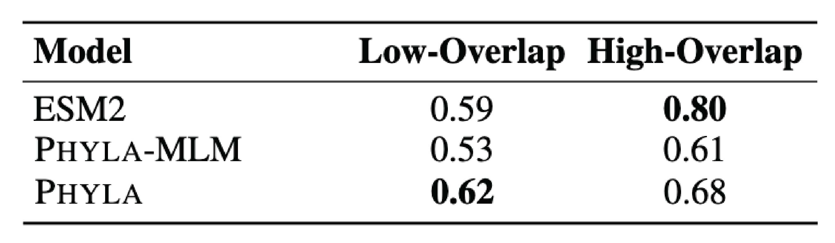Figure 7: Protein property prediction may be better aligned with comparison rather than reconstruction pre-training objective. The performance in protein classification on a more distant test set drops more for models that rely on the MLM loss (ESM2 and Phyla-MLM) than for the model that uses only the comparison loss (Phyla). The table was adapted from Table 8 of Ektefaie and Shen (2025), which is under CC BY 4.0 license.

Moreover, the comparison objective produces protein-level representations that are directly comparable to each other with simple distances (e.g., Euclidean). In contrast, the reconstruction objective optimizes for amino acid representations that a neural network head can decode. Thus, it does not directly optimize for meaningful distances between sequence-level representations, which are post-hoc derived from the amino acid representations (e.g., via mean-pooling) (Kelvin and Kubaczka, 2025; Tang, 2024).

Types of generalisation

Yasha distinguished between two types of generalization: different sequences (e.g., proteins with different functions) or different sequence characteristics (e.g., sequence length or the number of sequences in the comparison). While a lack of either is undesirable, the former is more problematic in practice, as it is less predictable for users (i.e., it is easy to know if a sequence is of the wrong length rather than biologically different) and harder to account for during pre-training (i.e., it is impossible to collect all possible sequence classes, but it is easier to train on sequences of different lengths).

While Phyla performs well in generalization across sequence types, Yasha noted that it, of course, cannot generalize to inputs with arbitrarily different sequence characteristics. For example, Phyla also struggles with extremely long sequences beyond the training length, as do many other sequence models. Thus, even if one had a sufficiently large GPU to embed such sequences, performance would be expected to degrade. Moreover, poor performance is also expected when reconstructing a phylogeny of many short sequences. Yasha mentioned that a potential reason for this could be the increased complexity of reconstructing a large phylogeny.

Finding new data to improve performance

Genomics data is “relatively” scarce. Many methods thus build upon new strategies for better leveraging the data⁶. For example, Alan first suspected that some of the previous attempts at fitting large ML models to GWAS had shattered due to suboptimal ML practices (e.g., misspecified training workflows). It was only later that he realised that using all available information (i.e., variant correlations) is crucial for making the models well-behaved. The importance of sufficient information sources surfaced again and again in all three conversations.

Epistasis is known as a challenging field for new biological discoveries. Boyang jokingly noted that if he had known how challenging the field was, he would not have entered it. The reliability of epistatic interactions is challenging to prove⁷, requiring very stringent testing protocols. His study subsequently identified only around a dozen epistatic effects across the whole genome - much fewer than when considering associations with individual genetic variants.

Boyang suspects that the testing power could be increased by better accounting for confounders. Currently, unobserved environmental effects are approximated based on genetic relatedness. In particular, if subjects share a large portion of their genome (e.g., similar genomic PCA embeddings), they may be related (e.g., within a family or geographic region) and thus share a similar lifestyle. However, there may be more effective data sources for modeling unobserved environmental effects, since relatedness is only weakly correlated with lifestyle. Boyang is currently exploring such alternative strategies. He has particularly high hopes for including other data modalities, such as gene expression.

The genomic variant matrices are not the biological ground-truth

Besides improving confounder adjustment, genomics research could also benefit from improving the genetic variant data itself. For example, when processing sequencing data, it may not be possible to correctly assign (i.e., map) variants (i.e., nucleotide bases) to genomic positions. This can occur in regions repeated across the genome. - If the sequence readout is shorter than the repeat itself (i.e., it does not cover any of the flanking non-repeated regions), it is impossible to determine from which of the repeats it originates. Thus, Alan highlighted the importance of using alternative sequencing methods with longer reads to disambiguate the genomic region of origin.

However, as long reads are not always available, it is worth considering models that can account for mapping uncertainty. As an example, Alan suggested using probabilistic models on short reads. - If there are two positions from which the variant could have originated, each of them could be, for example, assigned 0.5 variant probability.

Moreover, he also believes that using raw sequencing data directly has potential. He noted that the preprocessing used to obtain genotypic variant matrices (i.e., genomic positions × variants) from sequencing reads may lose some of the information present within the raw reads. For example, structural variants, where parts of the DNA are moved to a different position or lost, are generally hard to assign. Furthermore, the assignment is inconsistent across studies, both due to the underlying sequencing methods and the applied computational approaches (Jakubosky, 2020). Thus, if only variant matrices are used without the underlying data, it is often unclear if two distinct variants present in different studies may in fact be the same. As the transformation from reads to variants is a lossy compression that always “discards” some information, working directly with read data could improve variant effect detection.

Additional information sources also enable the study of biological questions that would otherwise go unexamined due to a lack of data. For example, in GWAS, rare variants are commonly disregarded because they are unlikely to yield significant hits, while at the same time reducing overall power due to the multiple-testing burden. However, when using genome-context-informed priors, phenotypic associations of rare variants become more likely to be discovered. Alan pointed out that for him, this is one of the most promising applications of the new prior.

Polarising views on useful priors, biases, and convenience in phylogenetic tree reconstruction

Sometimes, the extra bit of information may simply not be worth the effort of obtaining it, Yasha noted. His opinion factors in arguments on both convenience and questionable data quality.

Training Phyla requires pre-computed sequence relationships. The challenge with state-of-the-art phylogenetic tree reconstruction methods is that they are extremely resource-intensive and require custom settings for different sequence types, without clear heuristics for choosing them. Thus, using these methods for generating training data was out of scope.

Instead, he tested two approaches: a popular fast phylogenetic tree reconstruction method that reduces resource consumption through approximations and an approach that fully omits tree reconstruction. The latter simply uses the distances between sequences without information about how likely these differences are to occur during evolution (i.e., MSA-based distances*). The two types of training data performed comparably. This is quite unexpected, given that the latter does not account for the evolutionary probability of individual changes nor other evolutionary factors (e.g., the order of mutation accumulation). There are multiple plausible explanations for this, with arguments both on the side of lacking tree quality as well as how the trees are used in Phyla. Thus, I would not yet rule out the value of information potentially captured by high-quality phylogenetic trees.

However, a valid concern exposed by Yasha is that trees do not equal evolutionary ground truth. Instead, each tree carries strong biases from the author’s decisions about reconstruction parameters. Thus, individual trees used for validation each have different biases. In turn, the fast phylogenetic method used for generating training trees also has its own biases. Thus, the data without strong evolutionary assumptions (i.e., MSA distances) actually perform comparably. Yasha even pointed out that using an unbiased approach is preferable to training on data with specific methodological biases.

*The comparison was between FastTree 2, a phylogenetic tree reconstruction method, and MSA-based Hamming distance, which counts the number of differences between a pair of sequences in MSA. FastTree 2 also uses MSA as the basis for reconstructing a multi-sequence tree.

Let the data speak

A common way to let the model communicate potential data issues is through prediction uncertainty. At the same time, nonsensical predictions (i.e., negative variance parameters) are guarded against with strong priors or constraints. However, Boyang went a step further, using a fully unconstrained model, which is allowed to output nonsensical predictions if they better fit the data. He argued that, due to unknown covariates or interaction effects, it is often unclear exactly how the regression model should be set up. Thus, strong priors or constraints may introduce artificial biases that could override the information within the data.

In particular, his model can produce negative variance parameters (e.g., $\sigma^{2}_{g}$ , Figure 8). In practice, they observed a few cases where variances were significantly below zero. Boyang explained that this can indicate a misspecified model. - There may be missing interaction terms, either between variants and environment or for higher-order interactions between multiple genetic variants. Thus, they are further investigating these variants to determine whether any such interactions are actually present.

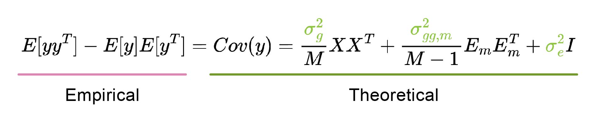Figure 8: Estimation of variance parameters σ². Boyang used the method of moments, which estimates the parameters (colored green) by equating the theoretical population covariance (containing the unknown parameters; underlined in green) to the empirical sample covariance (underlined in pink). The solution is obtained by solving the resulting linear system. If the theoretical population covariance equation is misspecified, the solution that best fits the empirical observations can result in negative variance parameter estimates. The theoretical covariance is derived from the marginal epistasis equation provided above, with covariate (C) effects omitted for simplicity.

Answering genomics questions with limited compute resources

While there are many ways to save on computing resources, not all of them work out in practice. Sometimes it is the performance that suffers, and in other cases, the hardware setup does not play nicely with the chosen method.

How flexible does the model need to be?

High model capacity requires more resources. However, in genomics, resource requirements often exceed a reasonable budget, calling for rationing. At that point, it is important to assess where cost-cutting could undermine the performance.

Alan highlighted a previous effort that sped up computation via low-rank approximation (i.e., truncated singular value decomposition) of the variant correlation LD matrix (Shi, 2026)⁸. He voiced concerns that this masks the effects of individual variants⁹. In particular, low-rank approximation groups variants with similar effects and represents them with a single factor (i.e., variants that exhibit a similar correlation structure with other variants across the genome). Thus, the effects will be averaged out, losing finer-grained resolution.

Instead, they set out to show that computational advances now enable calculations on the entire LD matrix without simplifications. Alan noted that it took quite a few failed attempts with different solvers before they found one that performed well. All in all, this would not have been possible without teaming up with his co-author Andreas - an expert in numerical linear algebra.

Yasha also initially set out to use a highly scalable method before it became clear that such resource cuts throttled performance. To enable the input of long sequences required for contrastive evolutionary modelling, he first tested state-space models (SSMs), as they scale better than transformers. In particular, while transformers scale quadratically with sequence length due to self-attention, the SSM Mamba scales linearly due to its recursive sequence memory, more akin to recursive neural networks (RNNs).

However, the SSM-only model did not perform well. It was only after combining it with attention blocks that the performance was good enough. The SSM blocks are, namely, less expressive. Yasha noted that their hyperparameter screen also recommended a combination of multiple SSM blocks with only a single attention block.

Another observation made by Ektefaie and Shen (2025) is that while a linear classifier performed well on top of embeddings from other protein sequence models¹⁰, it did not perform well with Phyla. Instead, they ended up employing an approach similar to nearest-neighbour classification, using neighbours within the reconstructed phylogenetic tree. Yasha explained that this may be required due to the specific geometry of the embedding space induced by the tree reconstruction loss. Tree structures, namely, lie in a hyperbolic (concave) rather than Euclidean (flat) space (Figure 9). Thus, a linear decision boundary that does not account for hyperbolic geometry (i.e., assumes Euclidean geometry) will not be a good separator.

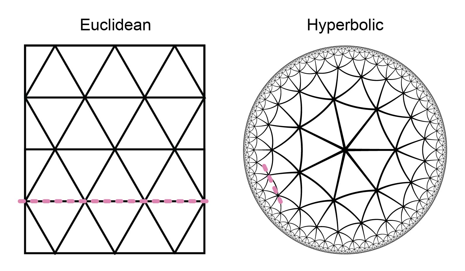Figure 9: Hyperbolic and Euclidean space. While Euclidean tessellation (e.g., {3,6} tessellation) can be separated with a linear decision boundary (pink line), this does not hold for hyperbolic tessellation (e.g., {3,7} tessellation). Tessellation notation {3,n} denotes a triangular pattern with n triangles at each vertex.

Overcoming resource constraints

Even when the model is set up, this does not mean it can be used right away. - Getting it to run on the local setup is a challenge of its own.

The main obstacle in Alan’s project was setting up the data loading. - He complained that getting data loading right ended up filling half of the project time. Their GWAS data consisted of a dozen million genetic variants, with variant correlation matrices that are squared that size. Besides the usual memory and efficiency challenges, such as the need to chunk up normalization or to access data consecutively based on the on-disk order, there were also many unexpected problems.

For example, some of the standard memory-mapped formats¹¹ did not work out of the box on their hardware, requiring extensive debugging of file system compatibility. On top of that, the I/O speed on the cluster varied depending on how occupied the I/O was by others. Thus, he wished that someone would develop a scalable GWAS data loader that could be used by anyone starting a new GWAS project.

Yasha also encountered cluster-related challenges. Their cluster contains different types of GPUs, and if you are in a hurry, you can not be picky about which one you get. However, since each of them has different resources, such as GPU memory, their workflows needed to be flexible enough to work on any of them.

Thus, they developed an adaptive system for determining the batch size (i.e., the total length of the input sequences). They trained a simple linear model to optimize the batch size for the current GPU. - At every step, the model suggested a maximal batch size, and the feedback on whether this led to an OOM error or not was used to retrain the model. While OOM errors slow down initial iterations, Yasha noted that the model can learn quickly, especially with reasonable initialization. Thus, they spent a bit more GPU resources but saved a lot of manpower. In addition, this setup may come in handy for new users who want to quickly try out Phyla.

Key takeaways

To make useful machine learning methods for genomics, it is not enough to know where current statistical approaches struggle. - One must understand what is actually important for broadening genomics knowledge. Without this, a newly developed method may solve one problem, but introduce others that make it unusable in practice.

References

• Amin and Potapczynski, et al. Training Flexible Models of Genetic Variant Effects from Functional Annotations using Accelerated Linear Algebra. ICML (2025).
• Barton, et al. The infinitesimal model: Definition, derivation, and implications. Theoretical Population Biology (2017).
• Candès, et al. Panning for Gold: ‘Model-X’ Knockoffs for High Dimensional Controlled Variable Selection. Journal of the Royal Statistical Society Series B: Statistical Methodology (2018).
• Dibaeinia, et al. PRSformer: Disease Prediction from Million-Scale Individual Genotypes. NeurIPS (2025).
• Ektefaie and Shen, et al. Evolutionary Reasoning Does Not Arise in Standard Usage of Protein Language Models. NeurIPS (2025).
• Fu, et al. A biobank-scale test of marginal epistasis reveals genome-wide signals of polygenic interaction effects. Nature Genetics (2025).
• Hemani, et al. Phantom epistasis between unlinked loci. Nature (2021).
• Huggins, et al. Reproducible Model Selection Using Bagged Posteriors. Bayesian Analysis (2023).
• Jakubosky, et al. Discovery and quality analysis of a comprehensive set of structural variants and short tandem repeats. Nature Communications (2020).
• Kelvin and Kubaczka, et al. NAND Hybrid Riboswitch Design by Deep Batch Bayesian Optimization. bioRxiv (2025).
• Morris, et al. Population phenomena inflate genetic associations of complex social traits. Science Advances (2020).
• Shi, et al. Contrasting the Genetic Architecture of 30 Complex Traits from Summary Association Data. The American Journal of Human Genetics (2016).
• Tang, et al. Pooling And Attention: What Are Effective Designs For LLM-Based Embedding Models? arXiv (2024).
• Tansey, et al. The Holdout Randomization Test for Feature Selection in Black Box Models. Journal of Computational and Graphical Statistics (2021).
• Zhang, et al. Floodgate: inference for model-free variable importance. arXiv (2022).

Footnotes

1. Some of the methodological details are simplified, not directly corresponding to the methods proposed in the papers, and the notation is adapted. ↩︎

2. Besides statistical power (e.g., reaching significance), a larger number of variants also reduces the estimated effect sizes. Assuming a certain overall genetic contribution to trait variability, this effect will be distributed across individual variants (i.e., model features). A higher-resolution genotype will thus have lower effect sizes at individual variants. This arises from several factors, including improved genome coverage (e.g., capturing additional causal variants whose effects might otherwise be misattributed to other variants) and noise (e.g., falsely attributing portions of the overall effect to non-causal variants). ↩︎

3. Linkage disequilibrium denotes correlation between the presence (i.e., inheritance) of genetic variants and subsequent correlation between their phenotype associations. Genetic variants located close to each other on the same chromosome are inherited together. This is in contrast to variants located further apart (e.g., on different chromosomes), which are randomly mixed when one of the two chromosomes is inherited from a parent. ↩︎

4. A quartet-based loss, inspired by classical phylogenetic tree reconstruction, was employed for contrastive learning. By determining which of the possible groupings of four samples into two pairs is the most likely, a tree can be reconstructed. The quartet is chosen for this task because it is the minimal set of samples that carries tree topology information. In particular, in a three-sample tree, there is only one possible topology for the tree if ignoring branch lengths and rooting (i.e., the relationship to the closest common ancestor, which would be the fourth sample). In contrast, the number of possible trees increases dramatically as more samples are considered, complicating the evaluation of the tree reconstruction task. ↩︎

5. Boyang explained that additive (i.e., non-epistatic) effects are often sufficient for predictive modeling. Thus, epistasis research primarily focuses on advancing biological understanding of genetic interactions. ↩︎

6. However, big datasets are on their own not enough, as described at the beginning of the section “Is machine learning trustworthy enough?”. ↩︎

7. Epistasis is hard to reliably identify as correlation of an unobserved factor (e.g., unmeasured environmental effect or non-genotyped variant) with a specific genetic variant can lead to false positive epistatic discoveries (Hemani, 2021). Namely, the effects of unobserved interactions may be falsely attributed to observed factors (e.g., epistatic pairs). Thus, Boyang explained that it is challenging to provide sufficient evidence about the reliability of the discovered interactions. ↩︎

8. In the original publication (Shi, 2016), the use of truncated SVD is motivated by retaining the largest singular values and vectors, which are assumed to be the true signal, and discarding lower ones, which capture noise. ↩︎

9. Note that while compression is guaranteed to lose some information, it was not tested in practice how much information is actually lost and how that affects results. Namely, since Alan and Andres reduced the cost of linear algebra operations below that of the neural network component, the speed gain from LD matrix compression was no longer relevant in practice. ↩︎

10. It is possible that nonlinear classifiers, such as the KNN classifier, may also improve the performance of other protein sequence models. However, this was not tested in the paper. ↩︎

11. Memory-mapped workflows keep the data on disk rather than reading it all into memory. They open a connection that enables fast access to on-disk data (i.e., for reading or writing). ↩︎