Matching flows to data

Expand all detail boxes for printing

Flow matching (FM) models learn a “data” flow between two distributions, which is subsequently used to generate one distribution from the other. While FM demonstrated remarkable success in diverse applications, the importance of aligning the FM algorithm with the data domain must not be overlooked.

For this blog post, I spoke with Alessandro Palma, Doron Haviv, and Lazar Atanackovic, all of whom utilized FM to generate single-cell gene expression (scRNA-seq) data. Through our conversations, it became clear that successfully answering biological questions requires careful adjustment of the FM algorithm.

Summary of the discussed papers

CFGen employs FM to generate scRNA-seq data under various combinations of biological and technical conditions. Special attention is given to generating data that closely resembles the distribution properties of raw scRNA-seq counts (Palma, 2024).

Wasserstein Flow Matching allows for the use of entire distributions (e.g., point clouds or Gaussians) as individual samples instead of single points. To achieve this, optimal transport (OT) maps are used as paths between sources and targets (Haviv, 2024a).

Meta Flow Matching predicts how individual observations will evolve based on the characteristics of the source populations from which they originate. To accomplish this, each source sample is conditioned on the embedding of the entire population it belongs to (Atanackovic, 2024).

As always, this blog post highlights topics that did not receive sufficient attention in the papers. If you are generally interested in FM for scRNA-seq data, I recommend reading the original papers, as many topics are skipped here.

While this blog post is based on discussions with Alessandro, Doron, and Lazar, I often omit their names for the sake of readability.

Sections list

• A brief introduction to flow matching
• What can be modeled?
  • Is the data sufficient?
  • Is this the right data representation?
  • Is the model up to the task?
• Why is the model not working?
  • Considering data scales
• A meaningful source
  • Diverse starting points for diverse samples
  • Starting with enough information
  • Keeping conditioning options open
• Finding the right paths
  • High-quality optimal transport paths for point clouds
  • Biologically meaningful paths
• Generating useful cells
  • Biological evaluation

A brief introduction to flow matching

FM is a sibling of diffusion models¹. It aims to learn a transformation of one distribution (source, p0) into another (target, p1). Consequently, we can generate new target samples by using the observed source samples as input to the FM model.

During training, FM learns the movement (velocity) of source samples at each step (time) along their path toward the target (Figure 1A). Specifically, the model approximates an ordinary differential equation (ODE) that transports the source to the target. To train the model, both target and source samples are required, with the latter often corresponding to random noise. The ground-truth path between the two is typically just an interpolation.

After training, new target samples can be generated by inputting source samples and iteratively updating their locations according to the velocity at each step (Figure 1B). To generate a specific type of target sample, the model can be conditioned on the desired target metadata (Figure 1A).

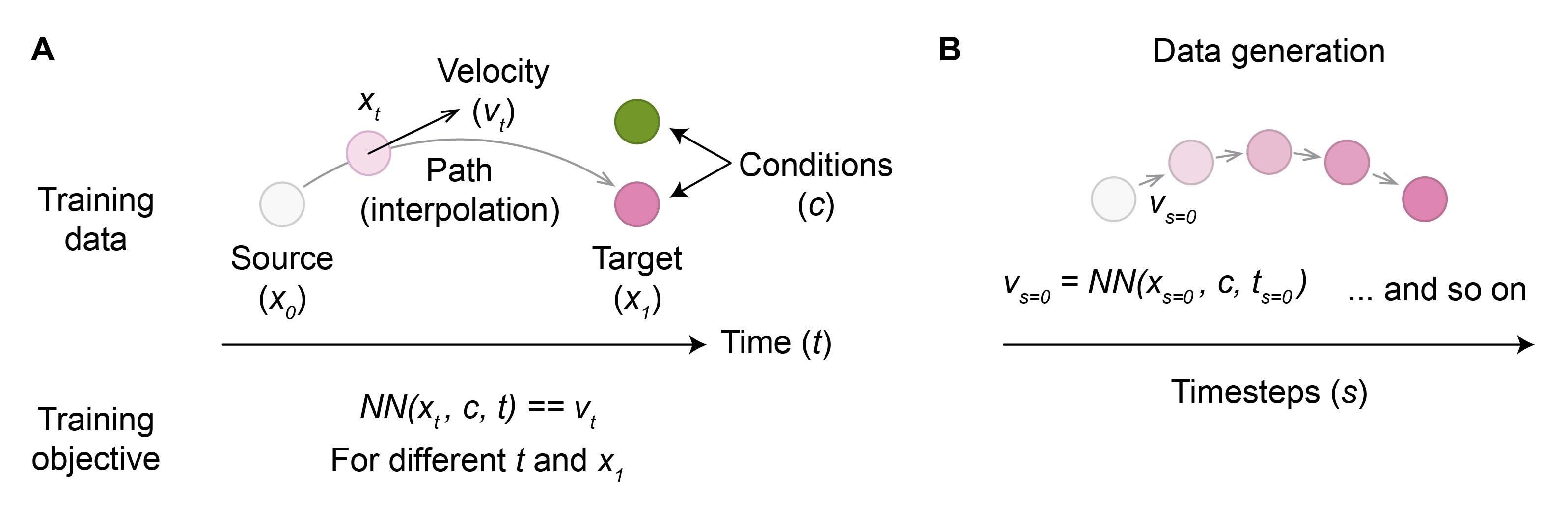Figure 1: Illustration of flow matching training procedure (A) and subsequent data generation (B).

Why flow matching?

While generative adversarial networks (GANs) used to be among the most popular generative models, FM and related modeling paradigms¹ have since won the race. In particular, GANs are notoriously hard to train due to their unsupervised training objective, which relies on the min-max game between the generator, aiming to generate realistically looking data, and the discriminator, aiming to classify the data as real or generated. Since both models are trained at the same time while competing against each other, the training is insatiable and requires a precise balancing of the two components. In contrast, FM models use supervised loss (Figure 1A), which is more stable. Besides, FM also has strong theoretical foundations, providing guarantees and inspiring more optimal algorithms.

What can be modeled?

Before starting to develop a new machine learning tool, we must evaluate whether the setting is reasonable from both the data and the modeling perspectives. If it is not, all the efforts may prove futile. - Regardless of how intriguing the proposed algorithmic advances may be.

Is the data sufficient?

As a first step, we must assess if the available data is sufficient to effectively model the desired process. For instance, one of the central questions in biology is predicting the outcomes of unseen perturbations or their combinations. Commonly used data consists of measured gene perturbation responses in cells (e.g., induced lack of expression through knock-out or silencing), which is available only for a subset of genes, and some general descriptions of all genes, such as their function in cell metabolism (e.g., gene set annotations). By combining this information, the aim is to predict how the cells will respond to perturbation of previously unmeasured genes.

However, the available information is often insufficient to provide practically useful predictions that could lead to new in-silico biological discoveries. In such a case, rather than throwing the latest model architecture at the data, it is preferable to identify a biological problem that is more likely to be solvable.

Missing information in biological data

Biological modeling is often constrained by biases and insufficient information contained within available datasets. Here are a few examples:

• Gene descriptors may lack informativeness:
  • Curated gene annotations from gene ontologies are frequently biased. They lack information about less well-known genes, resulting in blind spots. They are also enriched for more extensively studied cellular functions. This biases the derived gene similarities, neglecting less well-known cellular processes.
  • Experimental gene expression measurements across different tissues or cell lines may not provide sufficient information. For example, we may observe a few genes expressed exclusively within a single cell type, suggesting some kind of relationship. However, these genes can have very different molecular roles in that cell type. Thus, their perturbation could nevertheless lead to different responses.
• The diversity of the measured perturbation data is often too scarce to enable generalization. In the aforementioned motivating example, we may struggle to learn which gene features are genuinely informative and which are merely correlated by chance.
• The measured perturbation data may be highly noisy (McFarland, 2018; Corsello, 2020), and the number of replicates may be too low to deduce a clear perturbation effect.

Lazar shared that he also initially attempted to predict gene perturbation outcomes. However, he quickly realized that it is challenging to obtain sufficient data for generalization to new gene perturbations. - The mechanistic understanding of the genetic regulatory network is still far from being complete. Likewise, the gene representation models trained on gene co-expression and functional information are also often insufficient. Thus, he redirected his efforts toward a problem where he suspected a higher chance of generalization over input representations, as illustrated in the following paragraph.

We can reasonably assume that different patients will respond to the same drug in a somewhat consistent manner. - If that were not the case, the current drugs would be unusable. However, in practice, patients do vary in their responses to drugs. Nevertheless, there are often sub-populations of patients, allowing us to predict the outcome for a new patient given similar measured patients. As the patient outcomes are strongly influenced by individual patient characteristics, this task was more feasible to model than the gene perturbation example.

Is this the right data representation?

When setting up any generative model, we must first consider the intended use of the generated data. Without this consideration, the modeling may become unnecessarily complicated, or the generated samples may end up being over-simplified.

Cells within tissues are naturally represented as point clouds, which can be generated using Wasserstein FM. However, to find the OT map for Wasserstein FM in a computationally efficient manner, approximations must be employed. As discussed below, these are challenging to tune, and the OT solution may not converge properly. Additionally, samples composed of many individual points require more computing resources, as each point must be stored and modeled separately.

In some use cases, spatially positioned cells can be approximated by simpler representations, such as Gaussian distributions over neighborhoods² (Haviv, 2024b). Accordingly, the FM problem can also be simplified. In particular, transporting Gaussians instead of point clouds requires fewer computational resources, and the OT map has a closed-form solution that does not require fine-tuning the approximate solution.

Is the model up to the task?

FM models excel at conditional generation, effectively learning how diverse conditions and their combinations influence the data. However, this does not guarantee that they can truthfully generate the raw data itself.

A few tricks are needed to generate realistic scRNA-seq data with FM. To profile the expression within individual cells, the number of RNA molecules expressed from each gene is measured. This results in gene counts that follow a negative binomial distribution.

Neural ODE solvers, the core component of the FM generative process, can not generate count distributions. Transforming continuous source data to discrete target data would require discontinuous transformations. In contrast, neural ODEs are parametrized by neural networks, which rely on smooth activation functions that can not generate truly discrete data (Figure 2A). For example, consider two types of cells: one where the gene is expressed with a count of one and another where the gene is not expressed, resulting in a count of zero. While we could approximate this with a sigmoid activation function, our predictions will never be exactly one or zero. Instead, a common solution is to predict the parameters of the count distribution and sample the count data from it (Figure 2B) (Lopez, 2018).

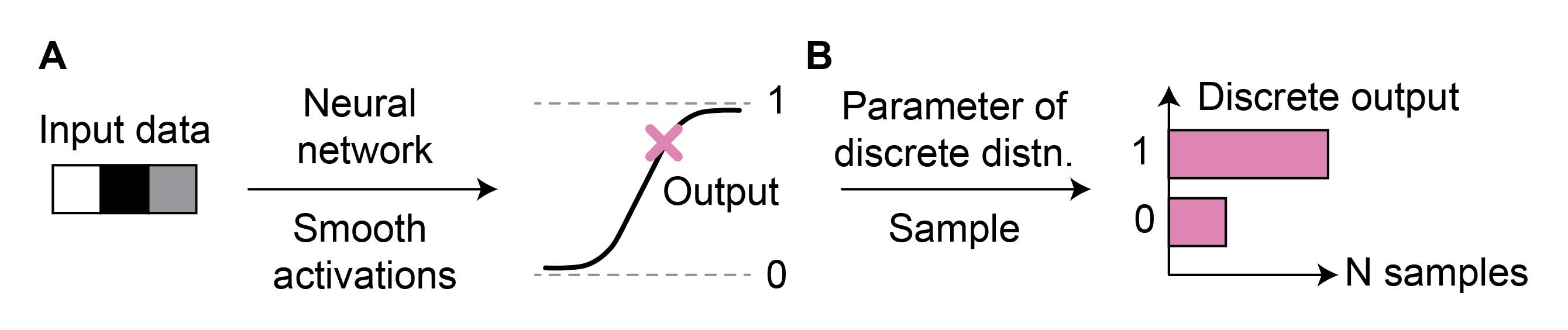Figure 2: Predicting counts with neural networks. Neural networks are parametrized by smooth activation functions, preventing them from directly outputting discrete data (A). Instead, the output can be used to parametrize a discrete distribution (e.g., negative binomial), from which discrete samples can be drawn (B).

However, in Alessandro’s experience, this did not overcome all the challenges posed by scRNA-seq distribution properties. The distribution of counts across genes is very sparse within a cell, as each cell expresses only a small subset of genes, while the rest have a count of zero. Moreover, the expression space is high-dimensional, with datasets typically having around 20,000 genes. Both of these properties proved to be challenging for FM models, which were less stable in higher dimensions and struggled to identify exactly which features (genes) should be zero. A solution to this challenge was to use an autoencoder to compress the data into a better-behaved lower-dimensional space, allowing it to be effectively modeled by FM.

FM as strong prior for autoencoders

Autoencoders excel at compressing and decompressing the data. However, the related generative architecture, the variational autoencoder, is not competitive in data generation. This limitation arises from the strong prior on the latent space, which is necessary for regularization. Without this prior, individual samples could be embedded in the latent space without meaningful relationships to each other. Accordingly, the generative process, which relies on sampling from the latent space followed by decoding, would be difficult to control. - Sampling two close latent points could result in vastly different outcomes.

Instead, FM can act as a more expressive “prior” on the latent space. As a strong conditional generative model, FM can generate meaningful latent samples. The autoencoder model can then decode them to produce the final data outputs. As FM can model complex unregularized distributions, additional latent space regularization is unnecessary when training the autoencoder. This leads to a more expressive latent space and enhanced decoding capabilities.

Why is the model not working?

Although an idea may look good on paper, its implementation often requires many tweaks. Thus, understanding the model’s behavior and its interactions with the data is key to success.

When attempting to solve a biological problem, it can be tempting to test the algorithm directly on the data of interest. However, it may be unclear whether the issue lies with the algorithm itself or the data. Biological data is often complex, and we may not fully understand its biases. Starting with synthetic data that captures the key characteristics of our problem will help us determine whether the algorithm works in principle. If it does, the next step is to find a way to pre-process the biological data to ensure compatibility with the algorithm.

Using the brain instead of compute power to optimize the model

Optimizing an algorithm by testing numerous hyperparameters is often impractical due to model complexity and long run times. Thus, we need to find a clever way of determining what is amiss. In his work, Doron initially used toy examples to fix standard parameters, such as neural network architecture and FM scheduler. He then focused on inspecting his new additions, such as the computation of the OT path. By analyzing the model outputs, he was able to identify the sources of errors. For instance, he observed that the generated points were averages of the entire target point cloud, indicating a collapse of the OT map, which is further explained in the following sections.

Last but not least, an important aspect of developing a new model is the availability of building-block libraries. In FM, a prime example is TorchCFM, which offers both FM code and comprehensive tutorials. Without such resources, re-implementing potentially beneficial modeling solutions becomes impractical, especially when chasing paper submission deadlines.

Considering data scales

Correct scaling of inputs and outputs was highlighted as crucial by everyone - Lazar, Doron, and Alessandro. In particular, neural networks perform best with data distributed around zero without extreme values.

This principle applies not only to the initial inputs but also to any intermediate representations passed to other parts of the network. For example, in meta FM, the population representations are trained on the fly, alongside the FM submodule. Nevertheless, the outputs of the embedding module are normalized before being passed to FM.

Moreover, explicitly scaling the data within the model to emphasize relative rather than absolute feature values can simplify the modeling task (Figure 3). For example, individual cells in scRNA-seq data exhibit significant variation in the total number of counts across genes, which is primarily a technical artifact. Cells with vastly different total counts can share similar biology and relative abundance of counts across genes. Although the model can be trained to predict the exact count number for each gene and cell, Alessandro found this approach led to less stable training. In contrast, the model performed better when separately predicting the relative expression across genes and a cell-specific scaling factor, which were combined to predict the final expression of every gene within a cell. This allowed the models to learn gene relationships jointly across cells, even if having different total counts.

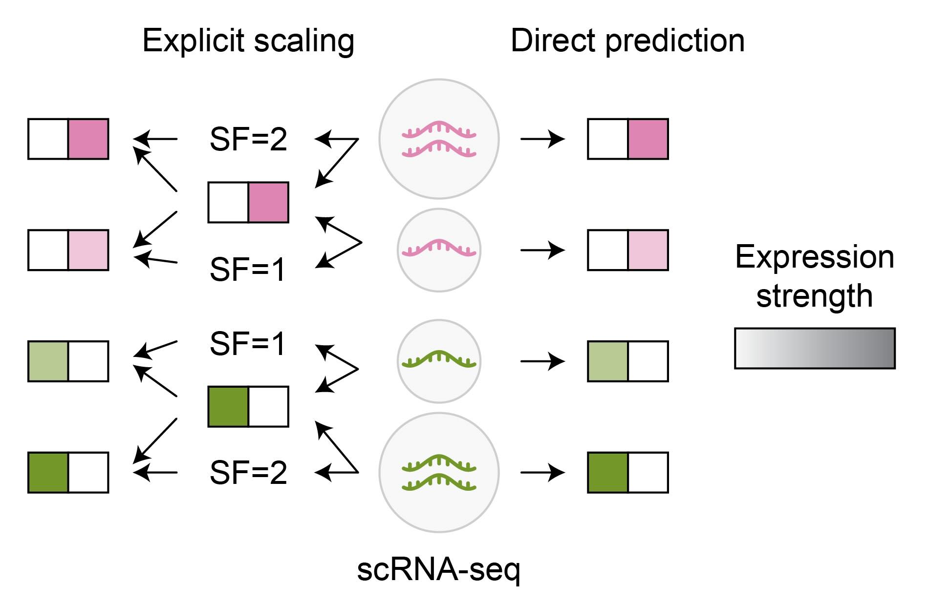Figure 3: Comparison of direct gene expression prediction and relative expression prediction, scaled with a size factor (SF). The latter facilitates information sharing among biologically similar cells (type of expressed gene, green or pink) that exhibit different technical artifacts (number of captured RNA molecules).

It is likewise important to consider the scales of the model outputs used for loss computation. For example, Doron observed that when comparing distributions, the gradients were dominated by either the mean or the covariance component of the loss³, neglecting to learn the other component. This behavior varied across data domains, prohibiting automatic scaling of the loss components. The issue was resolved by dividing the model into two separate networks, one learning the covariance and another the mean. This approach allowed both components to be learned reliably without interference from each other.

A meaningful source

The process of FM is often described as generating data from noise. However, to generate meaningful observations through ODE sampling, the quality of the source information, including any additional input conditions, is crucial.

Diverse starting points for diverse samples

To generate diverse samples, the sources must be genuinely diverse. This is straightforward when working with single-point observations (Figure 4A) as the source points can be directly sampled from the source distribution (e.g., noise). However, when generating point clouds, it is essential to ensure that the source point clouds are distinct, not just the individual points within them. Specifically, if we draw multiple groups of points from a distribution, all groups will tend to be very similar, following the sampling distribution (Figure 4B).

This can be addressed through two-level sampling (Figure 4C). First, the parameters of the distributions, each representing one point cloud, can be sampled. Then, these distributions can be used to sample the individual points.

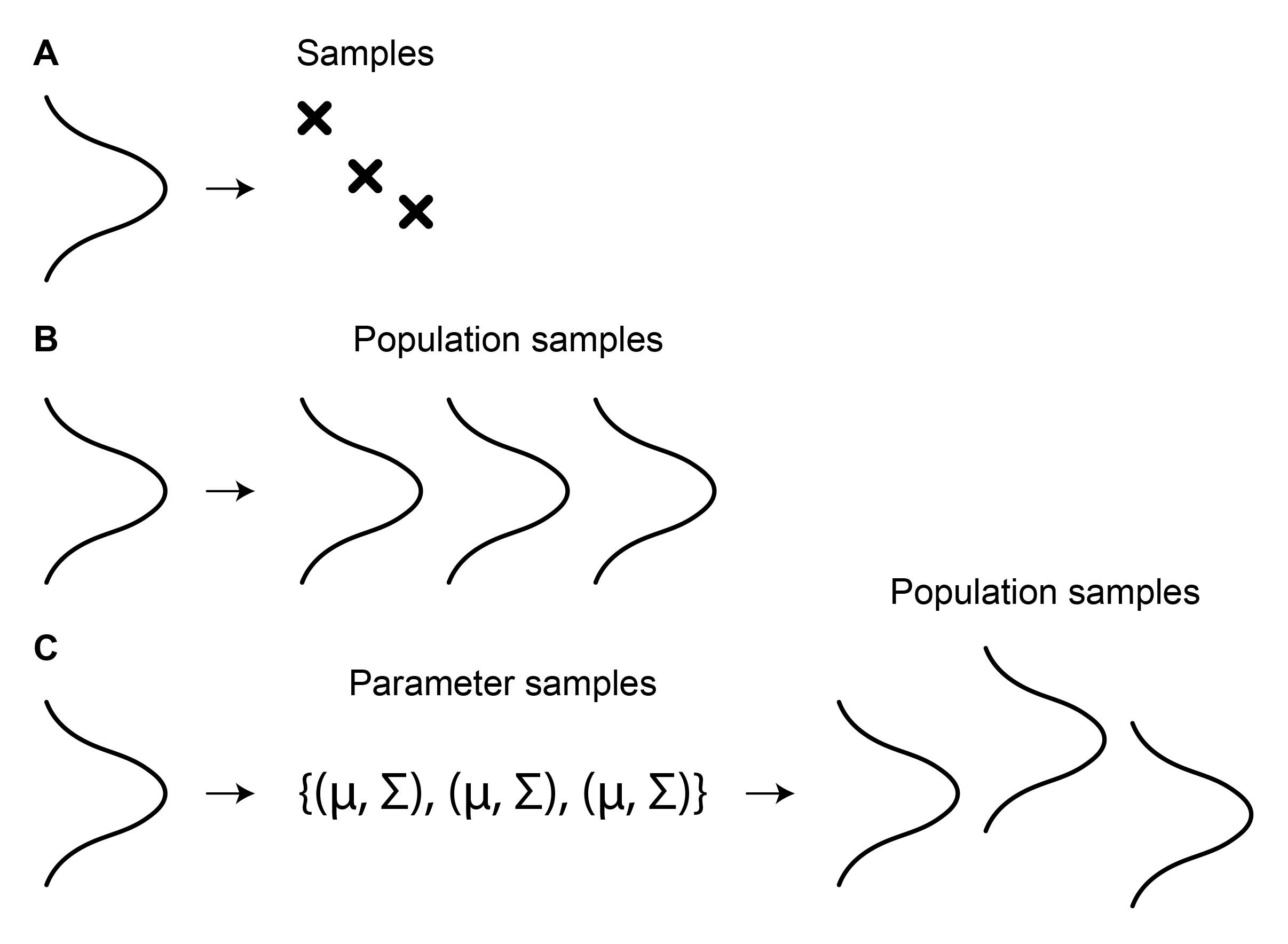Figure 4: Obtaining diverse source samples for FM inference. (A) Diverse point samples can be directly drawn from the source distribution. (B) When samples are themselves populations (e.g., point clouds), sampling N points from the source multiple times will yield identical distributions if N is sufficiently large. (C) To create diverse population samples, a distribution can first be used to sample parameters. These can then be used to parametrize distributions for drawing individual points for sample populations.

Starting with enough information

The FM task is limited by the informativeness of the conditions we use. For example, if we aim to predict how different cell populations will develop over time, the starting populations must already provide some indication of the end state. Therefore, we can not begin with arbitrarily distanced sources and targets, as a too-early source may not yet be determined towards a specific target.

Meaningful condition embeddings

When representing FM conditions with embeddings, such as in meta FM, they must capture relevant information. For example, when using source population for conditioning, the embedding must reflect both individual samples and the interactions between them. While it may be tempting to use pre-trained embeddings that generally describe the data (e.g., from emerging biological foundation models), these may lack the necessary details for the FM task unless they are fine-tuned.

It must also be assessed whether any technical factors influence the underlying nature of the data and can not be fully addressed by standard pre-processing methods, such as scaling. For example, in scRNA-seq the total number of gene counts within each cell is often viewed as a technical artifact related to the measurement efficiency. This effect is typically normalized using the size factor, which is inversely proportional to the total gene count. However, this effect can also be partially attributed to the cell size, which is linked to distinct biological properties. Consequently, if we generate a cell without knowing the size factor and then independently sample a size factor to scale the generated relative gene expression to counts, the cells will be unrealistic. Furthermore, this approach will reduce diversity, as the subtle biological variability captured by the cell size will be lost. Thus, a size factor must be used for both FM conditioning and final output scaling (Figure 5).

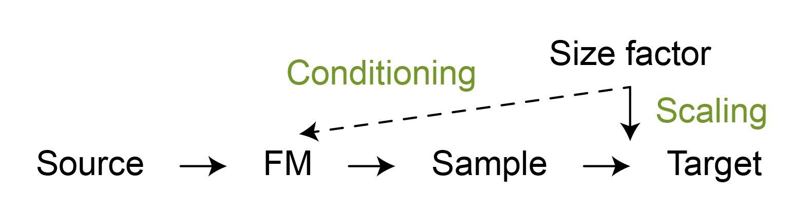Figure 5: To generate realistic samples, the scaling factors may also need to be conditioned on during FM inference besides being used for output scaling.

Keeping conditioning options open

One important aspect of conditioning is ensuring it is sufficiently flexible. For example, when working with scRNA-seq data, one might consider concatenating two standard conditions to the input: the technical batch and the cell type. However, this approach does not allow flexibility in matching different condition properties. - The model always requires one instance of batch and one instance of cell-type input features.

Instead, in CFGen, a separate velocity field is predicted for individual conditions, which are then summed into the final velocity for moving the data⁴. This enables flexible mixing-and-matching of conditions using a single pre-trained model⁵. For instance, we can decide to include only the batch condition, generating all cell types within that batch, or vice versa⁶.

Furthermore, individual conditions can be arbitrarily weighted. As an example, we may know that two batches had different stress levels during laboratory data preparation. Additionally, different cell types may vary in their susceptibility to stress. Thus, when generating the data, we could apply different weights to batch conditions depending on the cell type.

A note on choosing condition weights

While condition weighting increases flexibility, it also necessitates careful selection of the weights during generation. If the condition weights are too low, the generated data will resemble the unconditional case. - It will be widely distributed, matching the union of distributions from all conditions. Conversely, if the guidance is too strong, the variance in the generated data will collapse, failing to fully capture the target distribution.

Finding the right paths

The quality of the predefined paths between the source and target significantly impacts the training dynamics and the final FM model. A prominent example is the minibatch OT (Tong, 2024). While source points are typically randomly chosen, the minibatch OT demonstrated that pairing them with target points using an OT map straightens the paths (Figure 6). This stabilizes the training and accelerates the interference. While this technique is also popular in single-cell FM, additional considerations apply.

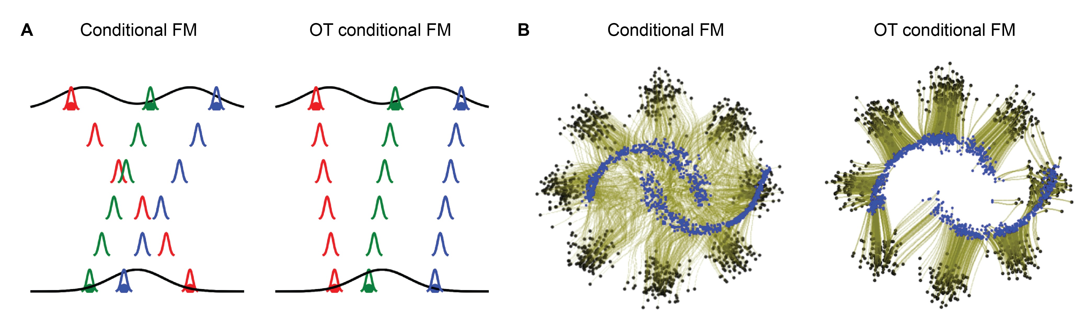Figure 6: Using OT to pair source and target samples during training, rather than pairing them randomly, simplifies the paths and, subsequently, FM (A). (B) Learned flows (olive green) from moons (blue) to eight Gaussians (black) using random (left) and OT-based (right) matching. The figure was adapted from Figure 1 of (Tong, 2024), which is under CC BY 4.0 license on OpenReview.

Choosing the correct distance metric for minibatch OT

When working with Alessandro and other colleagues on a different FM project, we observed that naively using OT between source and target can lead to nonsensical results if the distance metric is inappropriate. For instance, when matching distributions of male and female faces, using Euclidean distances between pixels may be effective, as it captures similarities in poses, hairstyles, and other attributes. However, in some cases, Euclidean distances between sample features do not adequately reflect the similarity relevant to the FM task. For example, cell images stained for different cell components, such as nuclei and membranes, can not be compared in this manner, as these components are located in different parts of the cell.

It is unclear how a meaningful metric could be defined a priori to match membrane and nuclei images originating from the same cell. Thus, I was considering learning the optimal source and target pairing alongside the FM training, with an approach similar to the attention mechanism. However, this was just an idea and I did not have time to test whether this approach actually works and outperforms random pairing. Nevertheless, distance functions have been previously learned on the fly in other settings, such as GANs (Salimans, 2018; Genevay, 2018).

High-quality optimal transport paths for point clouds

In Wasserstein FM, each path is defined as an OT map between the sample’s source and target distributions. Thus, the quality of the per-sample OT map is crucial. However, to avoid prohibitive runtime, the OT map must be approximated. This can be achieved with entropic OT, which is faster at the cost of a fuzzier OT map (Figure 7A). Namely, instead of matching each source point to the most suitable target, the source mass is more broadly distributed across the targets.

While the OT map may appear reasonable, this fuzziness can severely impact FM. Starting from a source point, the model learns to generate target samples that are interpolations of the matched targets, weighted by the OT map entries (Figure 7B). When generating 3D objects, this results in less sharp representations. The effect is even more detrimental in single-cell data, where the generated points no longer correspond to realistic cells. - They are a mixture of different cell types, which are biologically invalid. Therefore, the OT entropic regularization parameter must be carefully tuned.

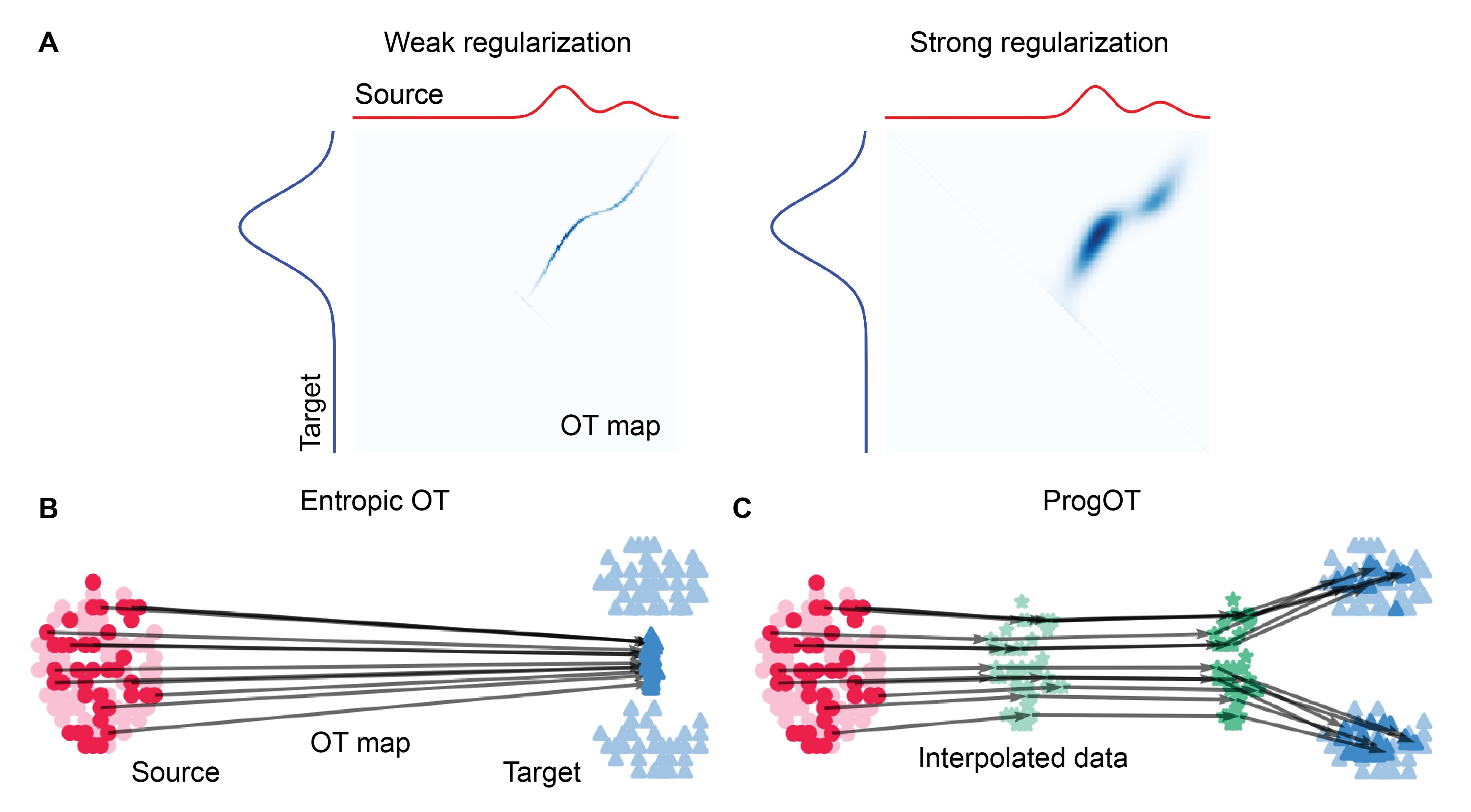Figure 7: Negative effect of OT regularization on FM. (A) Stronger OT regularization results in a less sharp OT map. (B) Using an entropically regularised OT map for FM leads to the collapse of the generated targets. (C) ProgOT mitigates the collapse by simplifying the OT problem into smaller steps. The panel A was adapted from Figure 1 of (Tang, 2024), which is under CC BY 4.0 license on OpenReview. The panels B and C were adapted from Figure 1 of (Kassraie, 2024), which is under CC BY-NC-SA 4.0 license on OpenReview. Please note that the original figures illustrated somewhat different scenarios.

Solving OT collapse with ProgOT

To address this challenge, Doron is currently exploring how Wasserstein FM could benefit from approaches that alleviate OT collapse, such as ProgOT (Kassraie, 2024). ProgOT (Figure 7C) divides the OT problem into smaller OT steps between the source and the target, which become progressively easier to solve as they approach the target. This allows for lower regularization in the later steps, enabling the correction of the final OT map.

However, while ProgOT alleviates the challenge of pairing with multiple target populations, it still results in local OT collapse. Namely, the pairing remains fuzzy within the matched target populations. When applied to scRNA-seq FM, the generated cells do not fully capture the variability of individual cell types, representing only an average of the sub-populations within each cell type.

Biologically meaningful paths

Commonly, the path between the source and target is an interpolation in Euclidean space (e.g., a direct line). While this produces realistic target samples, the intermediate samples obtained at individual points along this line may not be valid observations (Figure 8A). For example, if our data lies on a sphere, a direct line between the source and target would yield intermediate points that are invalid. Thus, when defining the path, the properties of the sample space (manifold) should ideally be accounted for⁷.

Figure 8: Defining biologically meaningful paths. (A) A straight line between two points on a manifold may not lie on the manifold itself. (B) A metabolic pathway, which is a sequence of chemical reactions that convert one metabolite into another, can be used to infer cellular states. In an early stage, a cell will have more metabolites at the beginning of the pathway, and over time, it will accumulate more terminal metabolites. (C) A comparison of straight paths between subsequent data snapshots and momentum-informed paths that may better reflect the true dynamics. The panel C was adapted from Figure 1 of (Chen, 2023), which is under MIT license on GitHub.

However, the biological data manifold is usually not pre-defined. Therefore, additional prior knowledge can be used to constrain the data paths:

• If the source and target are in sufficient proximity, the interpolation can be informed by metabolic dynamics (e.g., RNA velocity). Over a short time scale, the past and future changes in cellular metabolism can be inferred from the activity of successive reactions in a pathway⁸ (Figure 8B). This can help identify source cells that are more advanced in their development and target cells that are less developed, bridging the gap between the two populations.
• When data has been measured at multiple time points, it can be used to find paths that smoothly transition across the data points (Figure 8C) (Neklyudov, 2024; Chen, 2023).

Generating useful cells

A brief glance at machine learning conference papers and biological journal publications reveals a striking difference between the two formats: In machine learning papers, the method is the main focus, prominently described at the beginning, while the results are often relegated towards the end of the paper or placed in the appendix. In contrast, biological papers typically have an opposite structure, with methods often being skipped by the average reader. In summary, machine learning research emphasizes the ability to do something new, whereas biological research concentrates on uncovering new insights about biology.

This distinction was also highlighted during the interviews, based on the interviewees’ experiences in publishing both formats. For machine learning papers, a proof of concept is often sufficient. - Applying the method to derive new insights from the data is left for future work. In contrast, computational biology papers must demonstrate that the new method is practically useful. As a result, these methods are typically more closely tailored to the data domain. Additionally, a more rigorous evaluation is expected, as outlined below.

Biological evaluation

When submitting manuscripts to a conference venue, a standard set of metrics is applied to standard datasets to demonstrate that the new method at least marginally outperforms the current state-of-the-art. Such standardized evaluations increase comparability between publications and facilitate reproducibility. However, they often obscure method pitfalls that could significantly impact downstream applications. Fortunately, it is becoming increasingly common for reviewers at machine learning conferences to request more detailed and use-case-focused evaluations.

For a high-quality evaluation, we need to address several questions (Figure 9):

• Do the metrics accurately measure what we intend to assess?
• Are the chosen evaluation objectives truly meaningful for the downstream use cases?
• How to decide whether the result is “good enough”?

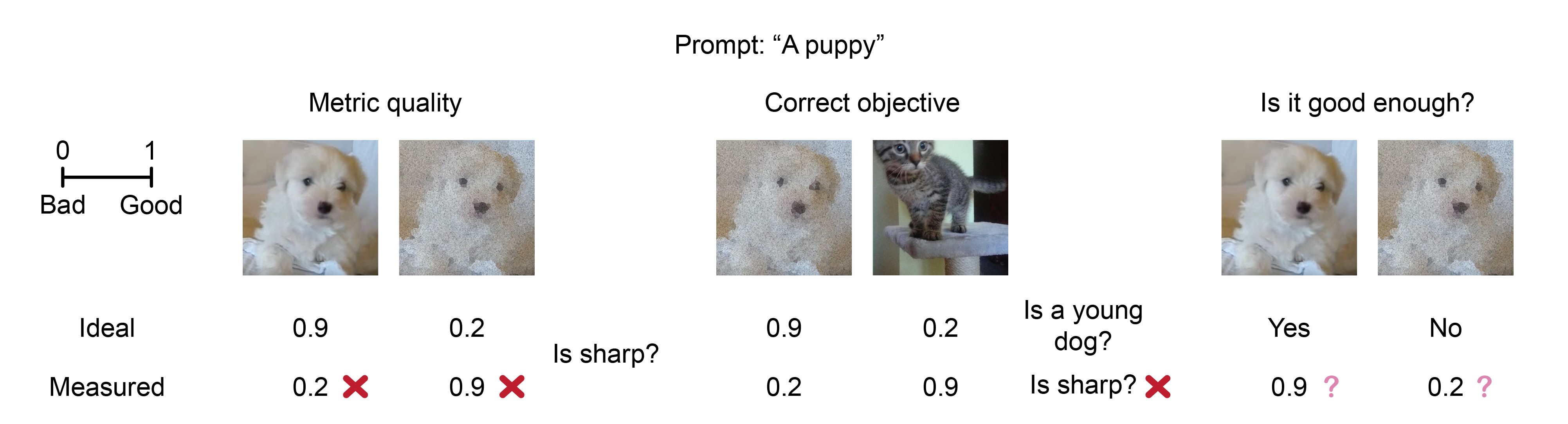Figure 9: Assessing whether the metrics evaluate the key properties of the data.

Metrics often exhibit unexpected biases. For instance, in my previous work on scRNA-seq representation learning, I found that some metrics are overly sensitive to output feature scales, resulting in scores that can be inverse to the true quality of the data for downstream applications (Hrovatin, 2023). Similarly, other biases in scRNA-seq representation metrics have also been reported (Lütge, 2021; Rautenstrauch, 2025). Thus, quantitative evaluation should be always complemented by qualitative evaluation (e.g., through lower-dimensional cell representations or expression of key genes) to ensure that the metric scores are meaningful.

Furthermore, it is not uncommon for metric objectives to be misaligned with the key data characteristics necessary for downstream use. For example, scRNA-seq representation learning metrics often evaluate whether cells can be separated by cell type. However, this largely neglects relationships between cell types and the heterogeneity of cells within each cell type (Hrovatin, 2023; Wang, 2024). This oversight can lead to incorrect biological conclusions. A common biological question involves identifying which cell types change in response to treatment, often resulting in slight distribution shifts within cell types. However, metrics that solely assess cell type separation will fail to capture whether sub-cell-type dynamics are truthfully represented in the generated data.

Preserving fine biological variation during FM

This issue was also highlighted by Alessandro. When the weight of cell type guidance was increased, the generated cells collapsed within their respective cell types. However, standard metrics did not detect this collapse, as they only assess whether different cell types are separated from one another.

He also raised concerns about the evaluation of FM for correcting technical batch effects. He inverted the FM procedure to generate noise samples from cells originating from different batches. Then, he used these noise samples to generate cells with a single batch condition, effectively eliminating technical differences. He employed metrics to assess whether the generated data reproduces the expected cell types. However, this approach does not ensure that cells from a specific cell subtype were correctly transported into the same subtype in the new batch. Namely, cells of a given cell type may be randomly shuffled with respect to the fine biological variation when transported to another batch. As a result, the information about sub-cellular variation may be lost or misrepresented.

Another common issue is the lack of interpretability regarding a specific error value. - Will the generated data be accurate enough to draw valid biological conclusions? For example, when comparing gene expression between two conditions, can we accurately deduce the key metabolic differences between them? Consequently, biological benchmarks often incorporate evaluations based on real downstream use cases.

Moreover, the metric may not reveal the source of the error. For example, in FM literature, the generated cells are frequently compared to ground-truth data by measuring the distances between the two distributions (e.g., using Wasserstein-2 distance across all features). However, these metrics have several limitations:

• We cannot determine whether the errors result from shifted or collapsed cell populations. In the former case, the data would still allow us to spot heterogeneity within the population. However, we would get an overall biased impression of the cell metabolism. In the latter case, the interpretation errors would be inverse.
• Errors may stem from minor differences across all genes or significant differences in a single gene. The latter can be more problematic, as it may lead to incorrect conclusions about the presence or absence of specific cellular functions associated with that gene. This contrasts with other domains, such as imaging, where substantial errors in a single pixel may be unnoticeable.

Other pitfalls in capturing distribution properties

When using non-distributional metrics (e.g., Euclidean distance) to compare a generated cell to a target (e.g., true population mean), additional biases may emerge. A specific distance value may have different relevance for different genes. Namely, some genes are less tightly regulated, leading to more noisy expression values where a larger error may be acceptable. Similarly, highly expressed genes typically exhibit greater variance. Thus, it is important to use metrics that account for the variability of ground-truth features.

We must also consider which distribution properties we need to capture. While point clouds of dots within a 3D object are shift-invariant, this does not hold for cells within a tissue. A car remains a car regardless of its position in space; the individual points can be located anywhere as long as their relationships are correct. In contrast, generating realistic cell populations within tissue space requires attention to the location of individual cells. Namely, each cell type has specific metabolic characteristics (e.g., gene expression) that must be captured.

When discussing the genuineness of generated cells, we must also consider the question: What is a valid cell? The biological space is theoretically vast, encompassing tens of thousands of omics features (e.g., genes or metabolites). However, only a small subset of it is biologically valid - that is, cells with such values exist in reality. Ongoing efforts to comprehensively profile biology across different organisms and environmental conditions are gradually contributing to answering this question. Nevertheless, the final answer likely lies in the distant future. Until then, finding ways to assess the usefulness of the generated cells will be key.

Key takeaways

While machine learning can facilitate new biological discoveries, it is key to consider which biological questions can currently benefit from these techniques and how the algorithms should be adapted to the data at hand. - In other words, prioritizing the data is key to developing useful methods.

Acknowledgements

Théo Uscidda and Dominik Klein suggested the references on learning distance functions on the fly.

References

• Palma, et al. Generating Multi-Modal and Multi-Attribute Single-Cell Counts with CFGen. ICLR (2025).
• Haviv and Pooladian, et al. Wasserstein Flow Matching: Generative modeling over families of distributions. arXiv (2024a).
• Atanackovic and Zhang, et al. Meta Flow Matching: Integrating Vector Fields on the Wasserstein Manifold. ICLR (2025).
• McFarland, et al. Improved estimation of cancer dependencies from large-scale RNAi screens using model-based normalization and data integration. Nature Commmunications (2018).
• Corsello, et al. Discovering the anticancer potential of non-oncology drugs by systematic viability profiling. Nature Cancer (2020).
• Haviv, et al. The covariance environment defines cellular niches for spatial inference. Nature Biotechnology (2024b).
• Lopez, et al. Deep generative modeling for single-cell transcriptomics. Nature Methods (2018).
• Tong, Fatras, and Malkin, et al. Improving and generalizing flow-based generative models with minibatch optimal transport. TMLR (2024).
• Salimans and Zhang, et al. Improving GANs Using Optimal Transport. ICLR (2018).
• Genevay, et al. Learning Generative Models with Sinkhorn Divergences. AISTATS (2018).
• Kassraie, et al. Progressive Entropic Optimal Transport Solvers. arXiv (2024).
• Tang, et al. A Sinkhorn-type Algorithm for Constrained Optimal Transport. arXiv (2024).
• Neklyudov and Brekelmans, et al. A Computational Framework for Solving Wasserstein Lagrangian Flows. arXiv (2024).
• Chen, et al. Deep Multi-Marginal Momentum Schrödinger Bridge. NeurIPS (2023).
• Hrovatin and Moinfar, et al. Integrating single-cell RNA-seq datasets with substantial batch effects. bioRxiv (2023).
• Lütge, et al. CellMixS: quantifying and visualizing batch effects in single-cell RNA-seq data. Life Science Alliance (2021).
• Rautenstrauch, et al. Metrics Matter: Why We Need to Stop Using Silhouette in Single-Cell Benchmarking. bioRxiv (2025).
• Wang, et al. Metric Mirages in Cell Embeddings. bioRxiv (2024).
• Bilous, Hérault, and Gabriel, et al. Building and analyzing metacells in single-cell genomics data. Molecular Systems Biology (2024).
• Lipman, et al. Flow Matching for Generative Modeling. ICLR (2023).
• Gao, et al. Diffusion Meets Flow Matching: Two Sides of the Same Coin. (2024).
• Yang, et al. Diffusion Models: A Comprehensive Survey of Methods and Applications. arXiv (2024).
• Zhou, et al. Fast ODE-based Sampling for Diffusion Models in Around 5 Steps. CVPR (2024).
• De Bortoli, et al. Diffusion Schrödinger Bridge with Applications to Score-Based Generative Modeling. NeurIPS (2021).

Footnotes

1. FM used to be promoted as an alternative to diffusion models due to its ability to sample from any source distribution, not just standard Gaussian, and the computational efficiency related to deterministic rather than stochastic sampling (Lipman, 2023). However, FM and diffusion models are two closely related concepts (Gao, 2024), and solutions proposed for one can often be transferred to the other. Various developments in the diffusion model field have alleviated the above-mentioned shortcomings (Yang, 2024; Zhou, 2024; De Bortoli, 2021). ↩︎

2. Note that groups of cells can be represented in many different ways. However, it remains unclear which approaches are best suited for specific use cases (Bilous, 2024). ↩︎

3. While standard FM models predict a velocity value for each sample (Figure 1A), the Wasserstein FM with Gaussians as samples predicts velocity distribution for each sample. These distributions are parametrized by mean and variance, hence the loss can be decomposed into two components optimizing the two parameters individually. ↩︎

4. To enable such conditioning, we must learn both the baseline unconditional vector field and the conditional fields that can be flexibly added to it. Ideally, we would have separate unconditional and conditional observations for this purpose. However, such data is unavailable as all observations come with associated conditions. Consequently, during training, each input is either combined with one of the available conditions or none. This enables the model to learn both unconditional and conditional vector fields. During the inference, the conditional samples are generated by nudging the unconditional vector fields toward the direction of the conditional ones. ↩︎

5. Arbitrary condition sets could also be integrated by embedding them into a single condition representation (e.g., using a transformer). However, this would not provide precise control over condition weighting. - While we could use weighting to create the embedding, this does not guarantee that the FM conditioning mechanism will correctly utilize this information. ↩︎

6. The paper proposed mixing different condition types, such as cell type and batch. However, an interesting avenue to explore in the future would be mixing different categories of the same condition type. For example, real scRNA-seq data often contains doublets, that is, observations where two cells were accidentally measured together, resulting in a mixture of cell types. One could attempt to generate doublets by combining the velocity fields of individual cell types. ↩︎

7. An example of Wasserstein FM, where the points remain on a sphere throughout the entire generative procedure, is provided in this tutorial. ↩︎

8. RNA velocity compares the amount of RNA that has not yet been processed for protein production to the downstream quantity of the processed RNA. When the amount of the unprocessed RNA is greater than the processed RNA, it indicates that the RNA was recently transcribed from the corresponding genes, leading to the production of the proteins encoded by those genes. This allows us to predict the direction in which the cell’s metabolism will develop. ↩︎